Introduction

When we began learning SQL, almost everyone of us started by using the wildcard operator: "SELECT * ..." It is incredibly convenient. It tells the database engine to fetch every single column from the particular table, and we don't have to type out every column name individually.

While "SELECT * .." is fine for quick troubleshooting or ad-hoc debugging on our local machine, using it in production application queries, especially when joining multiple tables together, can be one of the most common and dangerous anti-patterns in database development. It can quietly degrade the system performance, waste the server hardware, and cause critical application crashes.

In this article, we will use our local Microsoft SQL Server to break down exactly why "SELECT * .." in joins can be a silent performance killer.

Glossary

To understand how "SELECT * .." could impact the performance of our local database, we must first understand some of the key terminologies of the SQL Server engine.

Clustered index

A clustered index decides the actual order in which the table’s data rows are stored. Let's think of our table as a printed book. If the book is arranged alphabetically by customer name, then finding a customer by name becomes easier because the pages are already sorted in that order. That arrangement is like a clustered index. In simple words, a phone directory can be sorted alphabetically by last name, by phone number, or by city.

But the same printed phone directory cannot be physically sorted in all three ways at once. That is exactly why one database table can have only one clustered index. Usually, when we create a primary key, SQL Server automatically makes it a clustered index unless we specify otherwise.

Non-clustered index

A non-clustered index, on the other hand, is a separate lookup list that helps SQL Server find rows faster without changing the actual order of the table. We can think of it like the index at the beginning of a phone directory. The phone directory pages stay in their normal order (say sorted alphabetically by last name) but the index (or table of contents) has a list of mapping of every last name initial to a specific page number where from it starts. So, if we want to find “clustered index” in this phone directory, we do not need to read the whole book page by page. We can check the index (or table of contents), find the page number and jump directly to that page. A non-clustered index works the same way.

For example, let us imagine a bank customer database table. This actual database table may be stored in account ID order (clustered index, suppose it's a primary key). But we might often search customers in this database table by email address. So, SQL Server can create a separate non-clustered index on this email address column. That non-clustered index stores email addresses in sorted order and also stores a pointer to the full row in the main table.

Covering index

A covering index is a special kind of helpful index that already contains everything a query needs. So, SQL Server does not have to go back to the actual database table to get extra information. Let us assume that we are ordering a food from a menu card. Normally, the menu card only shows the item name and price. However, if we want to know the ingredients, calories and preparation time, then the waiter may need to go and ask it in the kitchen.

Now, let us imagine that the menu card already contains everything we need or might want to know:

• Item name
• Price
• Ingredients
• Calories
• Preparation time

In this case, the waiter does not needs to go anywhere else. The answer to every possible question is already available in the menu card. That is exactly what a covering index does.

Key lookup (or Bookmark lookup)

A key lookup is the extra work that the SQL Server has to do when an index does not contain all the data our query needs. Let us think of it like using the index (or table of contents) at the back of a textbook. The textbook index may tell us: “Bank transactions are discussed on page 52”. So we can quickly find the topic in the index. However, the index does not contain the full explanation. To read the details about bank transactions, we still have to turn to page 52. That extra step of going from the index to the actual page is similar to a key lookup. In SQL Server, this usually happens when:

1. SQL Server uses a non-clustered index to quickly find a row.
2. But our query asks for extra columns that are not stored inside that index.
3. SQL Server then has to go back to the main database table, usually through the clustered index, to fetch the missing columns.

For a small number of rows, this may not pose a big problem. However, if SQL Server has to do this for thousands or millions of rows, it would become highly expensive. It is like checking the textbook index, going to one page, coming back to the index, going to another page, and repeating this again and again. This would waste a lot of time and effort. This extra trip can use more disk space, available memory, and CPU usage.

Logical reads

Logical reads means how many small data pages SQL Server had to read to answer our query. The SQL Server does not usually read data one row at a time from the storage. Instead, it reads data in small fixed-size blocks called pages. Each page is 8 KB in size. We can think of it as like reading a notebook. If we ask someone to find one sentence, they may need to open several pages before finding it. The fewer pages they check, the faster will they finish. SQL Server works in a similar way.

When we run a query, SQL Server checks how many data pages it needs to read. These page reads are called logical reads. For example, if a query has to check many pages to find the answer, it has high logical reads. That usually means the query is doing more work and may be slower. If another query gets the same answer by checking fewer pages, it has lower logical reads. That usually means the query is more efficient. So, lower logical reads usually mean better query performance.

Setting Up Our Local Environment

Now that we have understood the basic key terminologies that we may be using in our article going forward, we can start setting up our local environment. To begin with local setup, we will need to create two tables: Orders and Customers representing a typical e-commerce relationship.

To create the tables, we can run the following script in our SQL editor:

CREATE TABLE Customers (
    CustomerID INT IDENTITY(1,1) PRIMARY KEY,
    CustomerName VARCHAR(100) NOT NULL,
    EmailAddress VARCHAR(150) NOT NULL,
    PhoneNumber VARCHAR(20),
    HomeAddress VARCHAR(250)
);

CREATE TABLE Orders (
    OrderID INT IDENTITY(1,1) PRIMARY KEY,
    CustomerID INT NOT NULL,
    OrderDate DATETIME NOT NULL,
    TotalAmount DECIMAL(18,2) NOT NULL,
    ShippingStatus VARCHAR(30) NOT NULL
);

In the Customers table, the primary key phrase automatically generates a clustered index, physically sorting the customers based on CustomerID. We need the Orders table so that later we can make use of this table in the JOIN operation and explain the danger imposed on using wildcard operator.

Next, we will create an optimized non-clustered Index on the Orders table. In production, tracking orders typically by CustomerID and OrderDate is incredibly common. This index will allow our SQL Server to quickly look up orders for a specific customer. To create the non-clustered index, we can use the following query:

CREATE INDEX IX_Orders_CustomerID_OrderDate 
ON Orders (CustomerID, OrderDate);

Now that we have our tables and index in place, we would need to insert high volume transactional data into these tables to mock the real time product database behavior. To do so, we will insert bulk records into these database tables. We can run the following queries from our SQL editor to insert bulk data and load our tables.

The following script populates the tables with sample data using high-speed recursive loops to provide enough physical disk rows so that a "Key Lookup" penalty becomes measurable.

-- 1. Insert 5,000 Mock Customers
WITH CustomerRows AS (
    SELECT 1 AS RowNum
    UNION ALL
    SELECT RowNum + 1 FROM CustomerRows WHERE RowNum < 5000
)
INSERT INTO Customers (CustomerName, EmailAddress, PhoneNumber, HomeAddress)
SELECT 
    'Customer_Name_' + CAST(RowNum AS VARCHAR(10)),
    'email_' + CAST(RowNum AS VARCHAR(10)) + '@company.com',
    '555-01' + CAST(RowNum AS VARCHAR(5)),
    '123 Mockingbird Lane, Suite ' + CAST(RowNum AS VARCHAR(10))
FROM CustomerRows
OPTION (MAXRECURSION 0);

-- 2. Insert 30,000 Mock Orders distributed among those customers
WITH OrderRows AS (
    SELECT 1 AS RowNum
    UNION ALL
    SELECT RowNum + 1 FROM OrderRows WHERE RowNum < 30000
)
INSERT INTO Orders (CustomerID, OrderDate, TotalAmount, ShippingStatus)
SELECT 
    (RowNum % 5000) + 1, -- Evenly distributes orders across our 5,000 customers
    DATEADD(DAY, -RowNum, '2026-06-22 00:00:00'), -- Counts backward in time from today
    50.00 + (RowNum % 500), -- Varies the order amounts dynamically
    'Shipped'
FROM OrderRows
OPTION (MAXRECURSION 0);

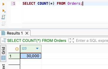
Once the above script is run successfully, all we need to do is to verify if there are 30,000 records inserted into the Orders table by counting the number of records in the table using the following query:

SELECT COUNT(*) FROM Orders;

The output should be similar:

The only final step we are left with is to enable the hardware telemetry to check the database performance metrics. To do so, we can run the following script. This will force our local SQL Server to output the detailed performance logs to the console by turning on the internal I/O (Input/Output) and CPU time counters. This allows us to inspect exactly how many storage pages were read under both query styles (problem and solution).

SET STATISTICS IO ON;
SET STATISTICS TIME ON;

Understanding the Business Requirement

First, let us try to understand a real time business scenario that we are trying to solve as a part of our hands on in this article. A very common business case scenario is that suppose we want to run a query to generate a report for a specific customer (say for customer with CustomerID = 2500) showing their name and their historic orders.

The easiest way to fulfil this business requirement is to use the traditional query style which we learn during our initial days. Here we make use of the "SELECT * .." clause which can prove to be dangerous when we take a look into the database performance metrics.

The following query generates the report but impacts the database performance. The query combines columns from CUSTOMERS and ORDERS where the IDs match. Since we wrote "SELECT *",  the SQL Server is legally forced to output every single column from both the tables. This demonstrate how "SELECT *" breaks all the indexing strategies and forces a heavy performance toll on our database engine.

SELECT *
FROM Customers c
INNER JOIN Orders o ON c.CustomerID = o.CustomerID
WHERE c.CustomerID = 2500;

Once the above query is run successfully, we should see a similar output in the performance metrics tab:

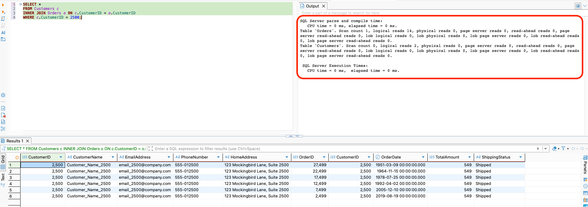
If we look at the performance metrics tab, we can see the text as:

Table 'Orders'. Scan count 1, logical reads 14...
Table 'Customers'. Scan count 0, logical reads 2...

We can understand the key lookup penalty we just faced here. In a highly tuned database, pulling orders for a single customer should take only 2 to 3 logical reads. While 14 pages might look like a small number because we only have 30,000 rows in our local environment, we will soon look at how it compares to the optimized version of this query and how the logical read drastically comes down.

Since we used SELECT * clause, the engine had to perform a key lookup. The SQL Server used our index to find the order records but then noticed it was missing other columns like TotalAmount  and ShippingStatus. The engine had to pause, jump over to the main database table and read those extra pages. This is why the logical reads jumped up to 14 in this case. If we scale this data volume from 30,000 rows to 3,000,000 rows in a real production environment, this query will scale linearly, jumping to hundreds or thousands of logical reads thereby causing a severe disk I/O bottlenecks and spiking our CPU usage.

A Performance Optimized Query

Now, let us change our strategy. Let us only request the exact columns our application screen or report actually requires to showcase in the final report. Instead of using the SELECT * clause, we will specifically mention the needed columns in the SELECT clause to see the change in the performance metrics.

To do so, we can make use of the following query. This query will retrieve order history for a specific customer by explicitly declaring the needed target columns. We are specifying the target columns during retrieval to prove how narrowing the column footprint allows the query optimizer to run at peak efficiency.

SELECT 
    c.CustomerName,
    o.OrderID,
    o.OrderDate
FROM Customers c
INNER JOIN Orders o ON c.CustomerID = o.CustomerID
WHERE c.CustomerID = 2500;

Once the query is successfully run, we should see the following performance metrics:

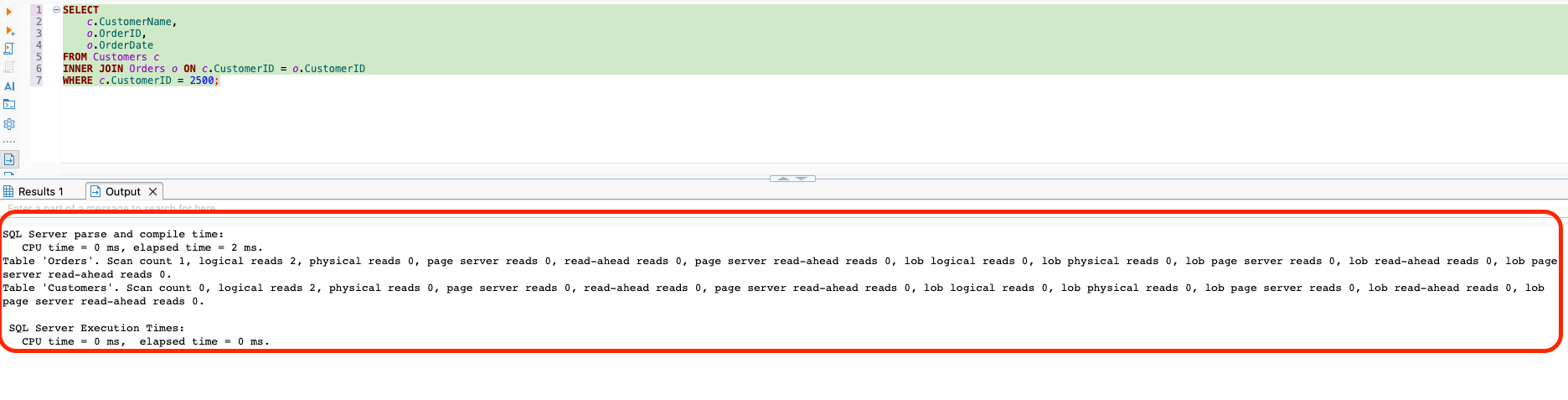
If we take a quick look at the performance metrics tab, we can see that:

Table 'Orders'. Scan count 1, logical reads 2,....
Table 'Customers'. Scan count 0, logical reads 2,....

Earlier, in the poor performing query with a "SELECT *" clause, the logical read on table Orders was 14 which has now come down to just 2 (proving it to be 85% less work done). When we changed "SELECT *" to only request OrderID and OrderDate , our SQL Server realized that it does not need to visit the main, heavily loaded Orders table on disk at all. Instead, it can straight go away to our non-clustered index (IX_Orders_CustomerID_OrderDate), which already holds those exact columns sorted perfectly by CustomerID. To find our data, the database engine only had to look at 2 memory pages (the root node of the index tree and the leaf node holding the data pointer). This is what we call a covering index.

However, at the Customers table, the logical reads remained 2 pages with a scan count of 0. This tells us that looking up a customer by their Primary Key (CustomerID = 2500) is already perfectly optimized via a clustered index seek. It jumps straight to the exact memory block where that customer's text name lives.

Conclusion

By replacing the wildcard operator (SELECT *) with specific columns needed to be retrieved/fetched, we transformed a query that forced a costly Key Lookup into a lightweight Covering Index search. In our local environment, this simple design change dropped logical storage reads on the Orders table from 14 down to just 2—an instantaneous 85% drop in system overhead. In a enterprise environment with millions of rows, this optimization saves gigabytes of RAM throughput and prevents server CPU spikes. The SELECT * clause introduces structural vulnerabilities that can crash our production software application entirely.

Also, when joining two tables that share identical column names (e.g., both tables containing columns named CreatedDate, ModifiedBy or Status), the "SELECT *" returns multiple columns with the exact same name header. Many application API parsers cannot handle duplicate key names in a JSON data response payload and might end up throwing an unhandled exception. Also, in our local environment setup, transferring data is instantaneous. But in production environment, our database server and our application server are usually in separate machines. If a table contains heavy data types like VARCHAR(MAX)  or image/file binaries, "SELECT *" forces megabytes of useless data to stream across our internal company network switch, slowing down the entire enterprise infrastructure.