

There is always a trade-off between speed and cost when provisioning cloud services. Typically, adding more virtual cores to go faster equates to more spending per month. There are several types of notebooks that are supported in Microsoft Fabric. For the lakehouse, we can choose either between Spark notebooks or Python notebooks. What is the difference between them?
Business Problem
Our manager has asked us to investigate how Python notebooks can save the company money. Many companies think they have big data. However, in most cases they do not have hundreds of terabytes of data stored in a lakehouse. Today, we are going to load the S&P 500 data for a 5-year period. This equates to 2553 comma separated values files with a total file size of 55.3 MB. We want to know the time and cost difference between using PySpark and Python notebooks.
Spark Starter Cluster
We can find the default spark settings for the workspace named ws-ssc-articles. It contains one executor node and up to ten worker nodes.
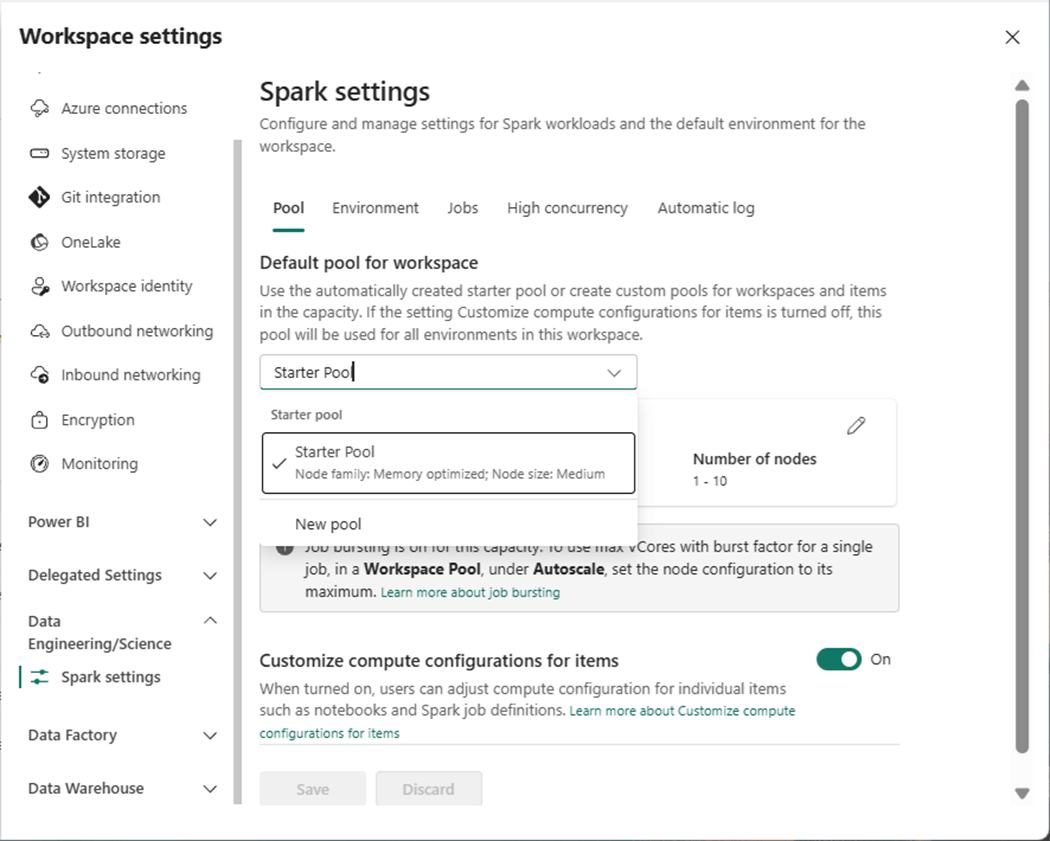
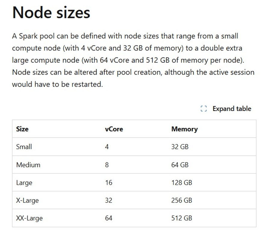
The above image shows the settings in my workspace while the image below was copied from MS Learn.
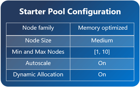
Each medium node has eight virtual cores and 64 GB of ram.
If we ask AI for the relationship between capacity units and virtual cores, we get the following answer.
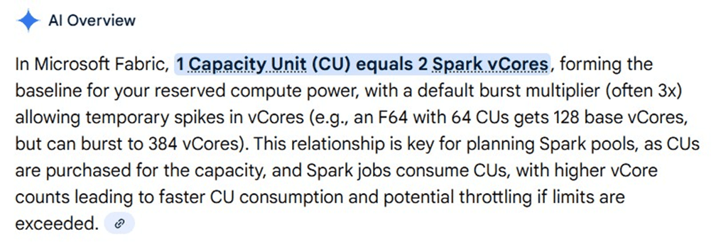
Every Fabric workspace should be associated with a capacity. In my case, the capacity named cpu4fabric is an F16 which has sixteen units of capacity or thirty-two virtual spark cores.
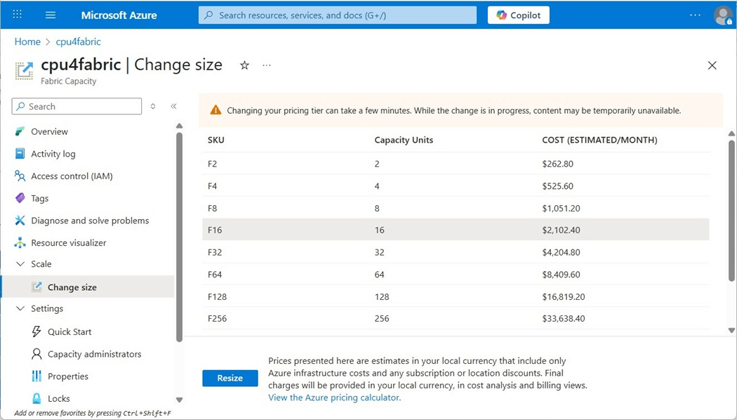
To recap, a spark cluster using two nodes will consume sixteen virtual cores or eight units of capacity. At that rate, we can only execute two notebooks at the same time using our current capacity settings.
Fabric Shortcuts
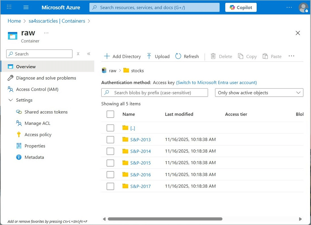
The quickest way to get data into the lakehouse is to use a shortcut. This connection allows the remote storage to look like local storage to the Fabric Spark Engine. The image below shows the storage container named sa4sscarticles contains five sub directories. Each directory is associated with a given year and has a comma separated values file with company stock data by symbol.
The image below shows two new shortcut types that are in preview. I will be exploring them in the future.
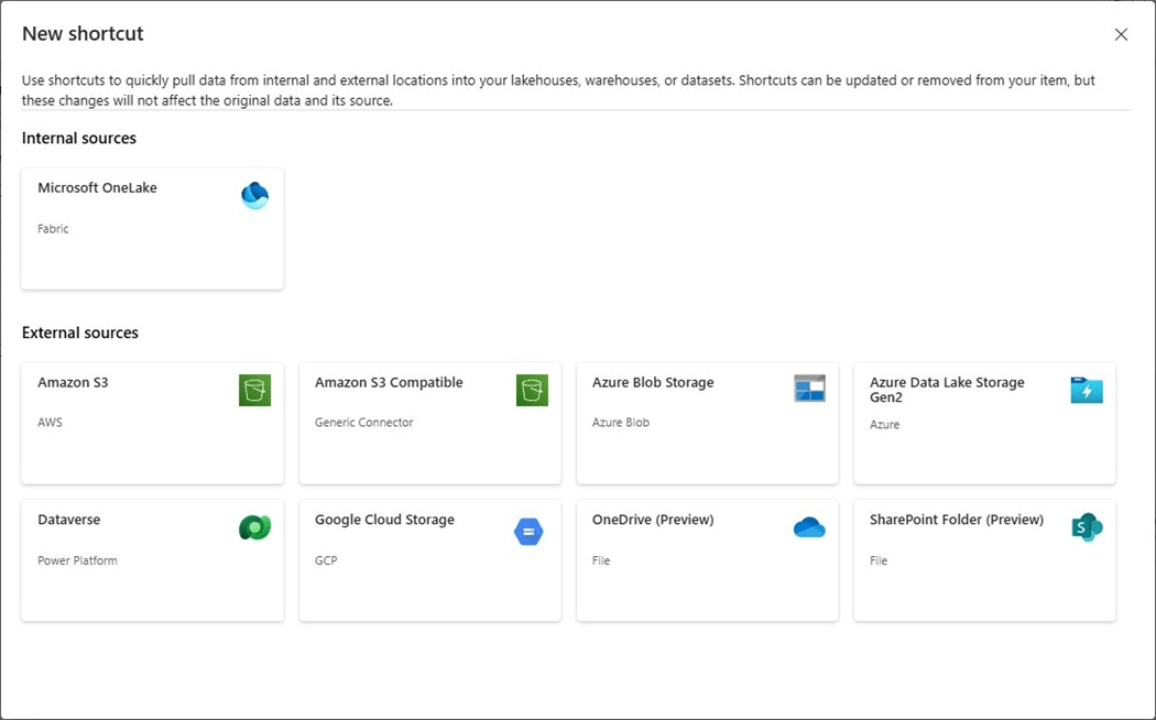
For now, let us create a new shortcut for Azure Data Lake Storage. To accomplish this task, we need to create a connection. The connection named ssc-articles-sa-raw must have some type of authentication. For testing, I am going to use my Entra Credentials.
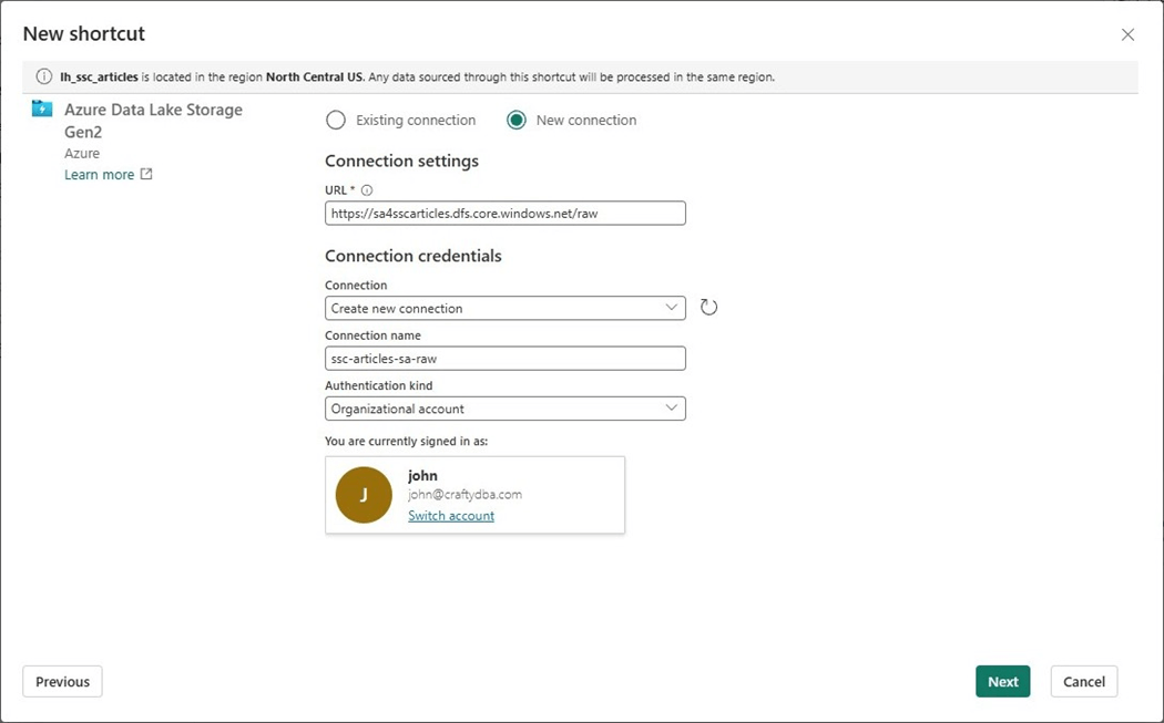
We can select which directory to shortcut into the lakehouse. Since we are working with stock data, please choose the obvious subdirectory.
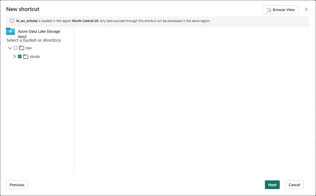
Click the create button to establish the shortcut.
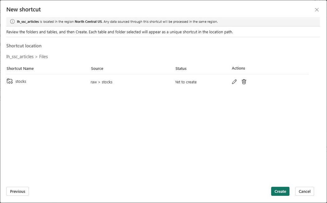
Now that we have the source data connected to the lakehouse files, let us create the schemas for the medallion architecture in the next section.
Lakehouse Schemas
I do not know why lakehouse schemas are still in public preview. This feature has been in that status for a while. If your company does not allow preview features, then produce a pre-fix that can be used for each stage. For instance, bronze (bz), silver (ag) and gold (au) can be represented by their abbreviation. Thus, a table name not using stages might be bz_stocks while the same table using schemas might be called bronze.stocks.
At this point in time, please create three schemas, one for each type of metal.
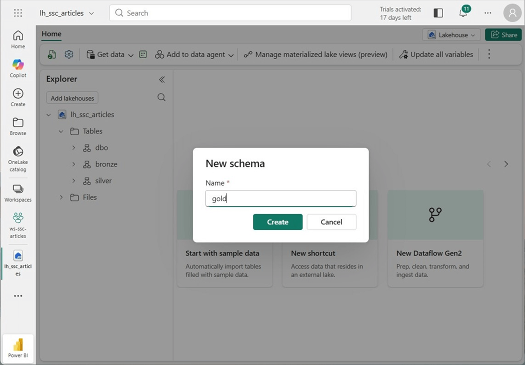
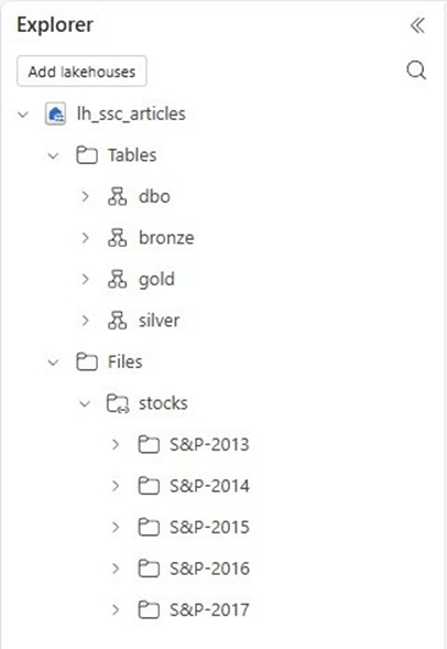
The final result is lakehouse with three medallion schemas and one shortcut to five years’ worth of stock data for the Standard and Poor’s listing of companies.
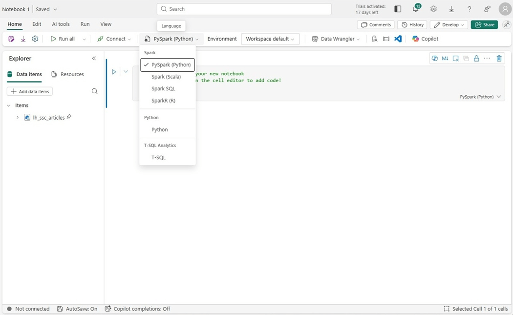
Spark Notebooks
Four different languages can be used to write spark programs. Today, we are going to write a PySpark notebook to ingest all the CSV files into a bronze table.
There are two ways to remove data from a Delta Table. One can use the drop table or truncate table syntaxes. Avoid the drop command if there is security or other features such as row level security using the SQL End Point. In this simple prototype, I am just going to remove and re-create the table. See code below to drop the given table using three dot notations for the fully qualified name.
#
#  1 - drop existing table (standard session - 7s)
#

df = spark.sql("DROP TABLE IF EXISTS lh_ssc_articles.bronze.pyspark_stocks")
display(df)
The code below reads in all the files recursively and writes them to the delta table.
#
#  2 -  use spark.read since it has the most options (standard session - 38s)
#

# include spark functions
from pyspark.sql.functions import *

# define path
path = "Files/stocks"

# define schema
custom_schema = """
    symbol string,
    date string,
    open decimal(12,4),
    high decimal(12,4),
    low decimal(12,4),
    close decimal(12,4),
    adjclose decimal(12,4),
    volume bigint
"""

# read in csv data
df1 = (
    spark.read.format("csv")
    .option("sep", ",")
    .option("header", "true")
    .option("inferSchema", "false")
    .option("recursiveFileLookup", "true")
    .schema(custom_schema)
    .load(path)
)

# get rid of file names
df2 = df1.filter(~col("symbol").contains(".CSV"))

# write delta table
df2.write.saveAsTable("bronze.pyspark_stocks")
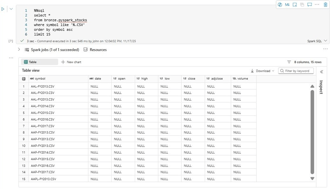
After comparing record counts, it was found that each file name was included as a row one or more times. My next question is what is the root cause of the file named ‘AAL-FY2013.CSV’ showing up three times?
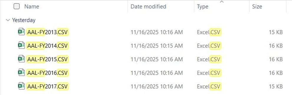
My first concern is the possible duplication of data. The stocks directory was copied from my laptop to ADLS Gen 2 using Azure Storage explorer. If we do a search of my local hard drive, we see there is no duplication of files. Thus, these bogus entries are being included by the PySpark engine. We can easily filter out these bad records before writing them to a Delta Table.
I will be showing all execution times after we complete our Python coding.
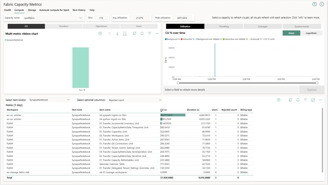
Capacity Metrics Application
The first place to look at capacity usage is to us this application. The application can be installed using the following link.
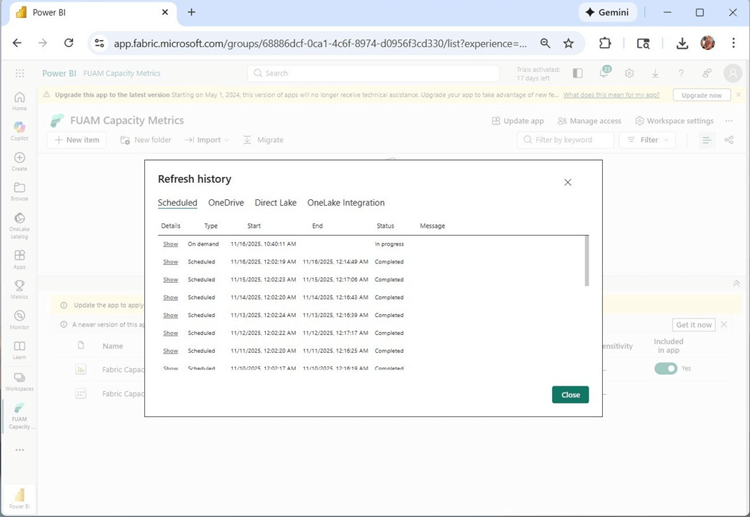
The problem with the capacity metrics report is that it need to be refreshed daily. Please make sure the dataset is schedule to be executed. The image above shows the manual refresh of the Power BI semantic model.
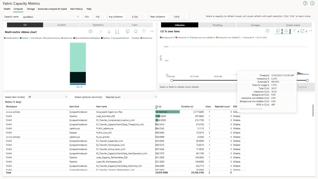
The application report shows capacity usage for the last 14 days and detailed items for the 30 days. I use this report as my first line of defense when trying to reduce spending. We can see that the interactive execution of the notebook named nb-pyspark-ingest-csv-files takes thirty-eight capacity units over a given time period. I filtered by hour and day to zero in on the data. Please note that our F16 on has thirty-two units of capacity.
Python Notebooks
While a spark cluster is good at parallel tasks, a python notebook is great when engineering small datasets. Before I write any code now adays, I usually create a prompt for a Large Language Model and start with the output as my code base. The function below reads all CSV files recursively and returns a pandas dataset.
#
#  1 - create function to read files recursively
#

import pandas as pd
from pathlib import Path

def read_csvs_recursively(root_dir: str, pattern: str = "*.csv") -> pd.DataFrame:

    # instantiate object
    root_path = Path(root_dir)

    # get file list
    csv_files = root_path.rglob(pattern)

    # empty list
    frames = []

    # for each file, read and append to list
    for file in csv_files:
        df = pd.read_csv(file)
        frames.append(df)

    # append each element
    if frames:
        return pd.concat(frames, ignore_index=True)

    # no file found case
    else:
        return pd.DataFrame()
The hardest part of coding is to know when to use an API path versus using a cloud path. Since this is just a python function, we need to supply the API path in the given call.
#
#  2 - execute the function (execution time = 1 min 50 s )
#

df = read_csvs_recursively(
    root_dir='/lakehouse/default/Files/stocks',
    pattern="*.CSV"
)
The delta lake library was built for the cloud. Therefore, we need to pass the fully qualified path to our table as input.
#
# 3 - write delta lake table (7 sec)
#

from deltalake import write_deltalake

# must be adls path
path = "abfss://e3479596-f0f8-497f-bcd3-5428116fa0ea@onelake.dfs.fabric.microsoft.com/926ebf54-5952-4ed7-a406-f81a7e1d6c42/Tables/bronze/python_stocks"

# over write
write_deltalake(path, df, mode='overwrite')
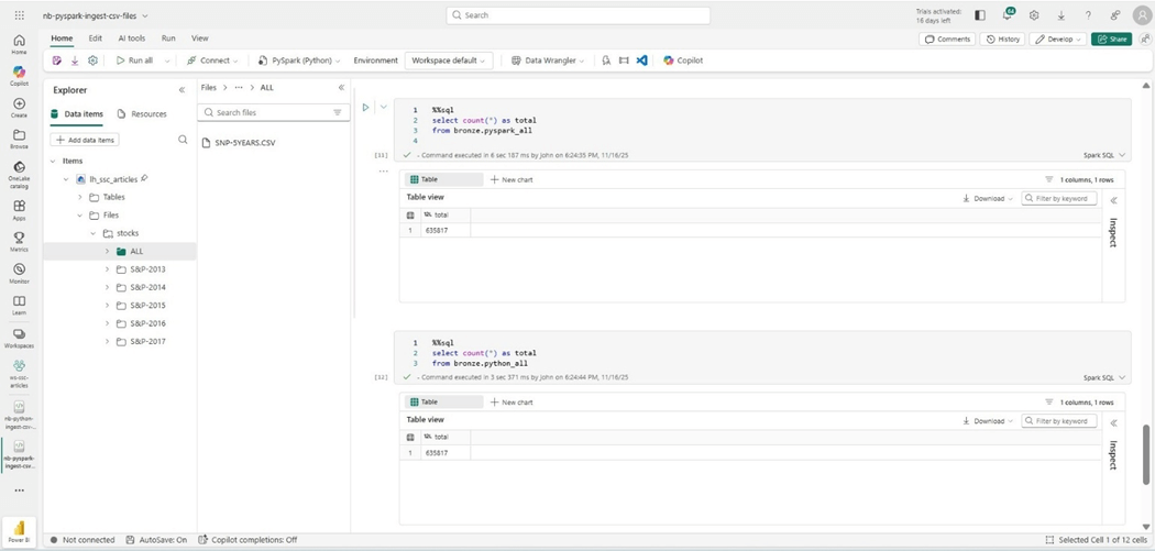
We know that the spark program will run faster if there is a large number of files to ingest. What happens if we combine all the files into one named SNP-5YEARS.CSV? The image below shows the newly staged files and a comparison between both tables. Regardless of program, we end up with the same number of rows.
Cost vs Speed
The table below shows how the Spark Cluster is extremely fast when it comes to a large number of files. However, it is slower when only one file is loaded.
| Notebook | File Count | Time Seconds | Capacity Units | Action
|
| Spark | 2533 | 11 | 10.4
| Drop delta table |
| Spark | 2533 | 38 | 10.4
| Read CSV files and write delta table |
| Spark | 1 | 11 | 10.4
| Drop delta table |
| Spark | 1 | 20 | 10.4
| Read CSV files and write delta table |
| Python | 2533 | 110 | 1 | Read CSV files into pandas dataframe |
| Python | 2533 | 7 | 1 | Overwrite delta table |
| Python | 1 | 5 | 1 | Read CSV files into pandas dataframe |
| Python | 1 | 2 | 1 | Overwrite delta table |
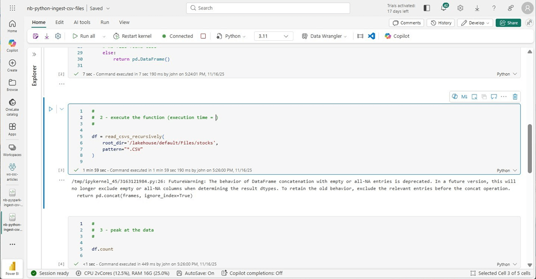
The cost of the python notebook can be calculated from the image below. Since we are using two virtual cores and sixteen gigabytes of memory, we know that the notebook only uses one capacity unit per second.
The capacity metrics application is helpful when determining overall cost by artifact. The spark notebook was executed for 78 minutes for a total of 48.7 K capacity units.
To recap, our F16 capacity has sixteen capacity units. That means a small company without large data can run sixteen python jobs in parallel at the same time. On the other hand, at most two spark jobs can run at the same time.
Summary
Do you really have big data? How fast do you need to load your data? Can you break a large process into smaller pieces to save money? These are some of the questions you need to ask yourself before deciding on using either Spark or Python notebooks. Here is a good article from MS learn detailing the differences between the two types of notebooks.
For smaller companies that have datasets that can be engineered with two virtual cores and sixteen gigabytes of memory, you can definitely do more with less. For instance, we ran one python job for 110 seconds to load 2533 files. If we can break this process down by year or sub-directory, the same data load of five hundred or so files should be less than 22 seconds. We would need to write a simple job to truncate the table before running code using append instead of overwrite mode.
Today, we just touched the surface of how to use Python notebooks in Fabric. Next time, I am going to talk about how to use the T-SQL magic command query SQL endpoint using Python. Both the Polars (fast dataframes) and Duck DB (in memory database) libraries are installed on the Virtual Machine used by Python Notebooks. These libraries open up what can be done with Python notebooks. Finally, working with REST API calls and in cloud databases are usually a requirement of a data engineer.
Enclosed is the code bundle for this article.