

In this article the COUNT function will be viewed from three aspects:
- The different ways of using COUNT
- The potential performance issues related with COUNT
- COUNT usage as an aggregated function (demo example)
COUNT is among the most used functions in T-SQL codes. Because of that fact, it must be well understood by developers. COUNT returns the number of the items/rows in a group. COUNT works like the COUNT_BIG function. The only difference between the two functions is their return values.
The following query returns a count of 863,345,304,648.
SELECT COUNT_BIG(*)
FROM       sys.all_columns A
CROSS JOIN sys.all_columns B
CROSS JOIN sys.all_columns C
The number is bigger than 2,147,483,647 which is the maximum value the integer data type can accept. And the next query
SELECT  COUNT(*)
FROM       sys.all_columns A
CROSS JOIN sys.all_columns B
CROSS JOIN sys.all_columns C
is failing with an error message that is telling that the conversion to the int data type could not happen.
Msg 8115, Level 16, State 2, Line 1
Arithmetic overflow error converting expression to data type int.
COUNT_BIG is aimed for the big counts.
Different ways of using COUNT
Ten ways of using COUNT are analyzed by trying simple queries on a temporary table in the example below.
SET NOCOUNT ON;
IF OBJECT_ID('tempdb..#TmpCounts') IS NOT NULL
       DROP TABLE #TmpCounts;

CREATE TABLE #TmpCounts
(Column1 varchar(20), Column2 varchar(10));

INSERT INTO #TmpCounts(Column1,Column2)
          SELECT 'Text1', NULL UNION ALL
          SELECT NULL, 'CText2' UNION ALL
          SELECT 'Text1', 'CText3' UNION ALL
          SELECT 'Text4', 'CText4' UNION ALL
          SELECT 'Text5', 'CText5' UNION ALL
          SELECT 'Text6', 'CText6';

/*(1)*/ SELECT COUNT(*) FROM #TmpCounts; -- 6 rows
/*(2)*/ SELECT COUNT(1) FROM #TmpCounts; -- 6 rows
/*(3)*/ SELECT COUNT(Column1) FROM #TmpCounts;  -- 5 rows
/*(4)*/ SELECT COUNT(ALL Column1) FROM #TmpCounts; -- 5 rows
/*(5)*/ SELECT COUNT(DISTINCT 1) FROM #TmpCounts; -- 1 row
/*(6)*/ SELECT COUNT(DISTINCT Column1) FROM #TmpCounts; -- 4 rows
/*(7)*/ SELECT COUNT('T') FROM #TmpCounts; --6 rows
/*(8)*/ SELECT COUNT(CONVERT(int, NULL)) FROM #TmpCounts; -- 0 rows
/*(9)*/ SELECT DISTINCT(COUNT(1)) FROM #TmpCounts; -- 1 row
/*(10)*/SELECT COUNT(NULL) FROM #TmpCounts
Query (1) returns the number of all rows (six in the example). COUNT(*) doesn't consider the duplicates; it counts all rows.
Query (2) returns a count of six rows too. Here “1” is a constant and has nothing with the ordinal positions of the table’s columns.
Query (3) returns the number of non-nullables in Column1 that results with a count of five rows. The row with a NULL in Column1 is excluded in the count.
Query (4) also returns a count of five rows as Query (3). The default ALL applies the aggregate function to all values. Additionally, the both Queries (3) and (4) throw this descriptive warning message
Warning: Null value is eliminated by an aggregate or other SET operation
because COUNT is an aggregate function and NULLs are eliminated.
In Query (5), “1” is again only a constant. By having DISTINCT for the constant, the query will return a count of 1. The next similar query
SELECT COUNT(DISTINCT 2) FROM #TmpCounts; -- 1 count
will again return a count of 1, because there is nothing different, except the constant ("2") that doesn't have any meaning.
Query (6) will count four distinct values in Column1 as the value “Text1” occurs two times. Here DISTINCT is applied on the column's values which is actually the essential difference from previous query.
Query (7) does the same as Query (2) considering “T” as a non-nullable constant. In this case the constant is a string.
In Query (8),
SELECT CONVERT(int, NULL)
will return NULL and like in Queries (3) and (4) the NULLs (NULL is unknown, it's not a value) are eliminated by an aggregate operation so that the final result is 0 rows to be counted.
Query (9) will return a count of 1 because DISTINCT is applied on a constant; same as Query (5) but with a reversed order of the COUNT and DISTINCT functions. It won't return same as Query (6) because in (6) the DISTINCT is applied to the data of Column1.
Query (10) will fail with the following error message
Msg 8117, Level 16, State 1, Line 27
Operand data type NULL is invalid for count operator.
as NULL is not allowed as an input expression in the COUNT function.
The following example queries will produce the same result – a count of 6, as they get input expressions, various constants, like in Query (2) and Query (7).
SELECT COUNT(-5.0) FROM #TmpCounts;
SELECT COUNT(+5.0) FROM #TmpCounts;
SELECT COUNT('') FROM #TmpCounts;
SELECT COUNT($10.0) FROM #TmpCounts;
COUNT(*) works well for NULL-able rows, while COUNT(Column1) doesn't.
IF OBJECT_ID('tempdb..#TmpCounts2') IS NOT NULL
       DROP TABLE #TmpCounts2;

CREATE TABLE #TmpCounts2
(Column1 varchar(20), Column2 varchar(10));
INSERT INTO #TmpCounts2( Column1, Column2 )
          SELECT NULL, NULL UNION ALL
          SELECT NULL, NULL;

SELECT * FROM #TmpCounts2
Column1              Column2
-------------------- ----------
NULL                 NULL
NULL                 NULL

SELECT COUNT(*) FROM #TmpCounts2;
-----------
2
SELECT COUNT(Column1) FROM #TmpCounts2;
-----------
0
Both select statements have identical execution plans and different results.
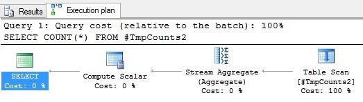
Figure 1. Execution plan of COUNT(*) on a table
The following calculations, which I think can be often found in some forms in codes, could produce different results too.
SELECT SUM(Amount) / COUNT(*) FROM MyTable
SELECT SUM(Amount) / COUNT(SomeColumn) FROM MyTable
These example queries for COUNT are essentially important to understand and have them in mind when you use the function or when combining it with other aggregated functions. COUNT can produce different counts depending on the way how it's used. COUNT is performing excellent on data objects that store a relatively small amount of data. For big tables it could cause some issues.
Which Is Faster: COUNT(*) or COUNT(1)?
Some say that COUNT(1) is faster than COUNT(*), or the opposite. For this question I made a simple test on a table with 6.5M rows. Both queries got same execution plans and returned identical results. ID is the primary key in the demo table.
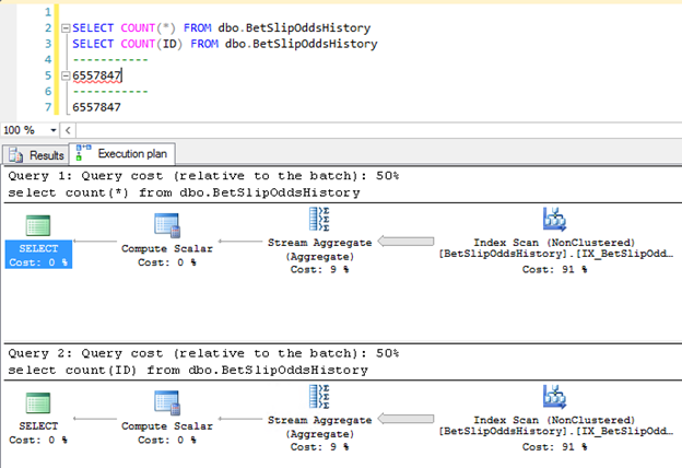
Figure 2. Results and execution plans of COUNT(*) and COUNT(ID) on a table
Let’s see the STATISTICS IO and TIME values. I allowed myself to clear the memory buffer because I was testing on a staging environment. That is definitely not recommended to do on production.
--DO NOT RUN THIS ON PRODUCTION!!!
DBCC DROPCLEANBUFFERS;
DBCC FREEPROCCACHE;
DBCC FREESESSIONCACHE;
GO

SET STATISTICS IO ON;
SET STATISTICS TIME ON;
SELECT COUNT(*) FROM dbo.BetSlipOddsHistory;
SET STATISTICS TIME OFF;
SET STATISTICS IO OFF;
GO
/*
Table 'BetSlipOddsHistory'. Scan count 1, logical reads 45670, physical reads 4, read-ahead reads 45665, lob logical reads 0, lob physical reads 0, lob read-ahead reads 0.
SQL Server Execution Times:
CPU time = 1344 ms, elapsed time = 1655 ms.
*/
--DO NOT RUN THIS ON PRODUCTION!!!
DBCC DROPCLEANBUFFERS;
DBCC FREEPROCCACHE;
DBCC FREESESSIONCACHE;
GO

SET STATISTICS IO ON;
SET STATISTICS TIME ON;
SELECT COUNT(ID) FROM dbo.BetSlipOddsHistory;
SET STATISTICS TIME OFF;
SET STATISTICS IO OFF;
GO
/*
Table 'BetSlipOddsHistory'. Scan count 1, logical reads 45670, physical reads 4, read-ahead reads 45665, lob logical reads 0, lob physical reads 0, lob read-ahead reads 0.
SQL Server Execution Times:
CPU time = 1436 ms, elapsed time = 1705 ms.
*/
Equal conditions were supplied for the both executions. The logical and the physical reads were identical.
COUNT(*) run with CPU time = 1344 ms that is a bit faster than COUNT(1) which run with CPU time = 1436 ms. The next time you may get slightly better results for COUNT(1) and so on. The answer is both queries perform the same.
From this example, you can see that the COUNT execution is not always a fast return of the count and in transact operations it could be a problem. A duration of 1500 ms is not an acceptable time in the quick-responsive systems and applications.
Counting the Rows of Big Tables
COUNT(*) is often used for counting the rows of a table. Nowadays, data is growing quickly and tables become big for short periods. Big tables have hundreds of millions of rows. Their size may be greater than 100GBs. Having a COUNT operation that executes excellent at a current time, may be a slow operation after some months of operations in a system. The COUNT on a big table could take long and impose blocking. For that reason we must be aware of some other approaches for obtaining the count info. One way could be the use of some dynamic views or functions to quickly obtain the number of the rows in a table. The dynamic management view sys.partitions and the OBJECTPROPERTYEX for example, can be used.
SELECT p.[rows]
 FROM sys.partitions AS p
 WHERE p.object_id = OBJECT_ID('Schema.TableName')
 AND p.index_id in (0, 1);

SELECT OBJECTPROPERTYEX(OBJECT_ID('Schema.TableName'),'cardinality');
The examples above will in most of the cases, return an accurate number of the rows in tables. This is perfect until the stats are up to date. The documentation for sys.partitions says that the rows is the approximate number. So the above are not a guarantee that it will always be accurate.
Big tables can easily get outdated indexes’ stats. Dirty reads at them can often happen due to many reasons. However, if you need an approximate number, then there are the DMVs data and functions. If you want an accurate count of the rows then you can use COUNT(*). But that could be a problem for the heavy tables: first it introduces locking and blocking and second its duration could not be acceptable. Using the hint (NOLOCK) for the reasons of decreasing the locking is not a guarantee that the actual number of rows will be returned.
There are some other approaches for the counting of the rows in big tables. See for example this article by Aaron Bertrand. In a part of his article he discusses the Indexed view.
CREATE VIEW dbo.view_name
WITH SCHEMABINDING
AS
  SELECT
    customer_id,
    customer_count = COUNT_BIG(*)
  FROM dbo.table_name
  GROUP BY customer_id;
GO

CREATE UNIQUE CLUSTERED INDEX ix_v ON dbo.view_name(customer_id);
Indexed views are usually created by specific purposes and they work fast. However, remember that it is almost same as having a physical table because the view's data is materialized. The gain is usually achieved by materializing a smaller volume of data so that the counts are obtained quickly and accurately.
Sometimes count operations are done unnecessarily. Overlooks happen in practice, especially when we make changes or develop wide and long codes. For example, the following query that is often used in codes,
IF (SELECT COUNT(*) FROM dbo.table_name WHERE <some clause>) > 0
can be replaced with
IF EXISTS (SELECT 1 FROM dbo.table_name WHERE <some clause>)
This could be a great performance improvement for the T-SQL codes especially when it's applied on big tables and possibly multiple times in a programmable object.
What Index is Used When Using COUNT?
If the table has no indexes (hash), then a full table scan is used in the execution plan (see Figure 1). If the table has indexes, then the query processor would use one of them.I’ll continue to test with the temporary table #tmpCounts, by executing the following code to populate data and create an index on it.
TRUNCATE TABLE #tmpCounts;
INSERT INTO #TmpCounts(Column1,Column2)
SELECT LEFT(name,20),CONVERT(VARCHAR(10),max_length)
FROM sys.all_columns;

CREATE NONCLUSTERED INDEX nix_Col1 on #tmpCounts(Column1);
Enable execution plan generation at this point and run the next query.
SELECT COUNT(*) FROM #TmpCounts;

Figure 3. Execution plan for COUNT(*) when an index is used
Now in Figure 3, you can see that the execution plan is different and the Non-clustered index nix_Col1 is used. The query processor decided to use the index. It's the same execution plan if we use COUNT(Column1).
If there are more indexes than the query processor will choose the one which is optimized to return the result. By using an index, less pages are read into memory, so that COUNT works faster. Having indexes on tables could help it execute faster.
When COUNT is used for subsets of rows, then filtering conditions constraint the volume of data to be processed. Again indexes are going to be of help, and especially the filtered indexes. Various filtering is actually an optimization of the COUNT operation. This is another topic that I only have to mention here.
COUNT as an Aggregate Function
COUNT is an aggregate type of function. It’s a deterministic function when used without the OVER and ORDER BY clauses. In the next example I’m going to use it in a grouping as a deterministic function. The next example shows how COUNT works with two different collations, and how COUNT is used for filtering.
Create a new table and populate with example data. My default collation is SQL_Latin1_General_CP1_CI_AS.
CREATE TABLE TmpCounts3 ( NAME VARCHAR(20) );
INSERT TmpCounts3 ( NAME )
        SELECT NULL UNION ALL
        SELECT 'Igor' UNION ALL
        SELECT 'IGOR' UNION ALL
        SELECT 'Branko';
The next query will list the results below. Note that it’s a good practice to put aliases when the aggregated functions are used.
SELECT NAME
      , COUNT(NAME) AS T1
      , COUNT(COALESCE(NULL, '')) T2
      , COUNT(ISNULL(NAME, NULL)) T3
      , COUNT(DISTINCT ( NAME )) T4
      , COUNT(DISTINCT ( COALESCE(NULL, '') )) T5
    FROM TmpCounts3
    GROUP BY NAME;
Output:
NAME T1 T2 T3 T4 T5
-------------------- ----------- ----------- ----------- ----------- -----------
NULL 0 1 0 0 1
Branko 1 1 1 1 1
Igor 2 2 2 1 1
Warning: Null value is eliminated by an aggregate or other SET operation.
Now create a database with Case Sensitive (CS) collation.
CREATE DATABASE [CountTest_collation] COLLATE SQL_Latin1_General_CP1_CS_AS
GO
USE [CountTest_collation]
GO
Run the same insertion of data from above, and then execute the same select again.
SELECT NAME
      , COUNT(NAME) AS T1
      , COUNT(COALESCE(NULL, '')) T2
      , COUNT(ISNULL(NAME, NULL)) T3
      , COUNT(DISTINCT ( NAME )) T4
      , COUNT(DISTINCT ( COALESCE(NULL, '') )) T5
    FROM TmpCounts3
    GROUP BY NAME;
Output:
NAME T1 T2 T3 T4 T5
-------------------- ----------- ----------- ----------- ----------- -----------
NULL 0 1 0 0 1
Branko 1 1 1 1 1
IGOR 1 1 1 1 1
Igor 1 1 1 1 1
Warning: Null value is eliminated by an aggregate or other SET operation.
Three and four rows were returned respectively by the same SELECT statement for the data. The reason for that is the different CS collation of the two databases. A different collation can definitely lead to different results, especially when querying string data. Note that the row beginning with “IGOR” is ordered before the one beginning with “Igor” because ANSI(“G”)=71 and ANSI(“g”)=103. It's result of the default ordering by the NAME column.
You can avoid collation issues in queries by directly specifying a collation next to. People are simply less used to it, and it may cause other issues possibly.
COUNT with HAVING is always used after GROUP BY. The bellow statements can be applied on the select query from above.
/*1*/ HAVING COUNT(*)>1 --returns one row
/*2*/ HAVING COUNT(DISTINCT ( NAME )) > 1 --does not return any rows
If we append the first clause (1) to the select query, one row will be returned, and with the second clause (2) there won't be any rows returned. HAVING with COUNT does act as a filter.
An ORDER BY clause can be used explicitly in the end as well. In that case the COUNT is not deterministic. See Deterministic and Nondeterministic Functions for more.
Conclusion
COUNT is easy to use by everyone. It should be used carefully because it could often not return the desired result for you. The counting duration could be unacceptable for an application. It's safe and fast to use COUNT directly on small tables or on temporary tables that usually have controlled subsets of data with a reasonable number of records. For big tables it worths to find alternatives for achieving the goal. Sometimes a price must be paid.
COUNT is used in aggregate operations and can be combined with other aggregate type functions as well. The last example, showed how a different database setting could result to different result sets. The considerations for the different ways of using COUNT shall be taken in with the aggregate operations too.
