SQL Server uses statistics to create query plans that improve performance. When writing a query, there are rules that are easily followed as to when to use left joins, inner joins, etc. The Query Optimizer, on the other hand, uses statistics underneath the covers to decide how exactly to retrieve the data and return it to the user. If you run an identical query on two different databases with the same schema, one 500 MB and another 500 GB, you are likely going to get two different execution plans, even though you are joining the same tables. The execution plan is generated based off of the statistics.
Before getting into how SQL Server creates and uses statistics, we will cover the basics of a histogram. A histogram is a graphical way to represent a data distribution. A simple example of a histogram, created in Excel, can be seen below. In this example you have a group of 188 people and you want to divide them up into bins by age. There is a formula for bin width, but for this example I just chose even width bins. You can see there are 6 groups, or bins, along with the number of people that fall into each of those age ranges. The histogram is the chart below the data that shows the distribution of people in each age range. As you can see the range 26-35 has the largest number of people in it.
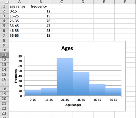
More information about histograms and their use can be found by searching on Bing/Google.
Now with a basic understanding of what a histogram is, it is time to move on to how this applies to SQL Server. Statistics are objects stored in a database about the distribution of data in a given field(s) in a table. Statistics are created in a few scenarios. The first is when indexes are created; statistics will be generated on the key column(s) of the index. Secondly, statistics will be generated for single columns that are used in query predicates when AUTO_CREATE_STATISTICS is turned on in the database. Finally, statistics can be created manually with a CREATE STATISTICS SQL command.
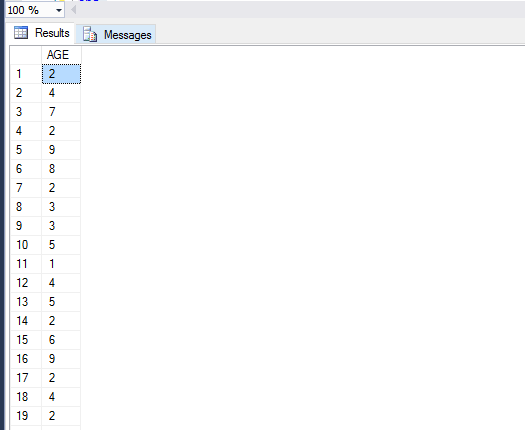
Now we will look at a basic example of statistics in SQL Server. First we are going to create a table called Ages and populate it with 188 records, which is the same number as in the example earlier in Excel. I am only making the age range between 0 and 10 so that the statistics on the table can be viewed more easily in this example.
IF EXISTS
(SELECT * FROM sys.objects WHERE object_id = OBJECT_ID(N'dbo.Ages', N'U'))
BEGIN
    DROP TABLE dbo.Ages
    ;
END
;
GO
CREATE TABLE dbo.Ages (AGE INT)
;
INSERT INTO dbo.Ages (AGE)
SELECT TOP 188 ABS(CHECKSUM(NEWID())) % 10 FROM sys.objects
;
SELECT AGE FROM dbo.Ages
;
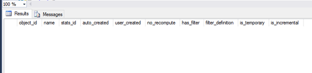
Now that the table is created, we can take a look at the sys.stats for this object. As you can see below, there are no statistics yet for this table because we did not create any manually, didn’t create an index, or use the column in a predicate.
SELECT
      object_id
    , name
    , stats_id
    , auto_created
    , user_created
    , no_recompute
    , has_filter
    , filter_definition
    , is_temporary
    , is_incremental
FROM  sys.stats
WHERE object_id = OBJECT_ID(N'dbo.ages', N'U')
;
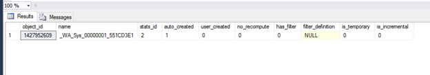
Now we can run a query against this table and use the only column in a predicate. Once we run this query, we can look at sys.stats again for this object and we see that there is now an entry.
SELECT *
FROM   dbo.ages
WHERE  age > 5;
SELECT *
FROM   sys.stats
WHERE  object_id = object_id(N'dbo.ages', N'U');
Now that we know the name of the statistic that was created, we can take a look at the actual information stored about the column in the Ages table using the DBCC SHOW_STATISTICS command like below.
DBCC SHOW_STATISTICS (N'dbo.ages', N'_WA_Sys_00000001_551CD3E1');
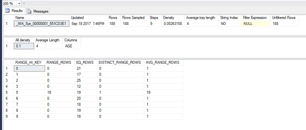
This command is going to return three result sets. The first result set is the header information with some basic information about the statistic such as name, when it was updated, number of rows sampled, etc. The second data set is the vector information this gives the density, which is 1 / distinct values, along with the average length in bytes, and finally the column name. The third data set, the histogram, is the most interesting and useful part of the statistic. I will go through each column and explain what each means.
- RANGE_HI_KEY – this is the upper limit of the range of values that fall within this step. So in this example, the first row has 0. Since all values in our table are positive that means that this step only contains the value zero.
- RANGE_ROWS – this is going to be the estimated number of rows that fall within this step but excludes the upper limit. As you can see most of the values here are zero except for RANGE_HI_KEY = 5 has some interesting results. As you can see there is no step for 4 in RANGE_HI_KEY, so 4 and 5 fall within the step with RANGE_HI_KEY 5. The 19 is referring to 19 records with a value of 4 in this step.
- EQ_ROWS – this is the estimated number of rows that are equal to the RANGE_HI_KEY value. In this example, there isn’t anything very interesting except RANGE_HI_KEY 5 again, it is estimated to have 19 rows with the value of 5.
- DISTINCT_RANGE_ROWS – this will be the estimated number of distinct values excluding the upper bounds. You can see in this example the only row with a value other than zero is RANGE_HI_KEY 5 and that is because, like mentioned earlier this step includes 4 and 5.
- AVG_RANGE_ROWS – this is calculated by RANGE_ROWS / DISTINCT_RANGE_ROWS for DISTINCT_RANGE_ROWS > 0
We have gone through the basics of what statistics are and how they are generated. The real importance of them is how the Query Optimizer uses them to choose whether an index is useful, an index scan or seek would be more efficient, etc. This is a more in depth topic that will be covered in the next article.