

The open-source version of Apache Spark is written in Scala. The issue with Scala (Object Oriented Java) is that fact that it executes slower than natively compiled code. Before there were language APIs for Spark, developers used to worry about resilient distributed datasets (RDDs) which are a read only sets of data items distributed over the computing nodes. The Dataframe API eliminated the need for dealing with RDDs and the SQL language allows developers to use relational knowledge on dataframes stored as temporary views.
In short, the PySpark language has simplified the data engineering process. How can we configure and tune the Fabric Spark Pool so that our programs execute faster on the same number of cores?
Business Problem
There are settings in the Fabric environment at the Tenant, Workspace and Notebook level that allow the administrator and/or developer to control how a PySpark program executes. Today, we are going to cover each setting that can be changed to tune your Spark program.
We need a rather large parquet dataset to perform this analysis on. The New York Yellow Cab dataset contains 1.5 Billon rows of data stored in 50 GB of parquet files. A simple PySpark program will be used to read the data into a dataframe, print the number of rows, and display the contents of the top N most records.
Spark Pool Configuration
Starter pools are one reason Microsoft Fabric gained popularity. Previously, a developer would have to wait two to five minutes for a cluster to start up before the job started execution. Instead, these pre-hydrated pools owned by Microsoft come up in mere seconds if the conditions are right.
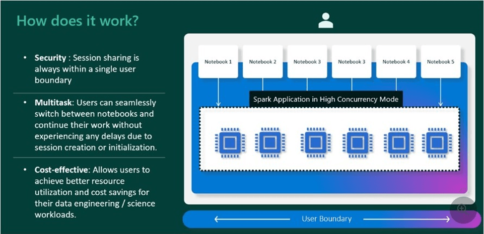
High concurrency sessions (clusters) support the idea that sharing is caring. Yes, the initial startup of a custom pool might be slow. However, additional workloads can re-use the cluster until it times out. Thus, the end user might see up to thirty-six times faster startup notebooks after the first session loads.
Finally, Microsoft has caught up with Azure Databricks by supplying the developer with a natively compiled execution engine. The Native Execution Engine (NEE) is based on Velox, a C++ database acceleration library, and Gluten, a middle layer which offloads Spark SQL execution to native engines for speed.
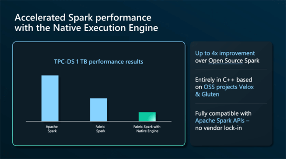
The above image shows impressive speed improvements with the Spark engine. Please note that all images are from Microsoft.
Spark Pool Configuration
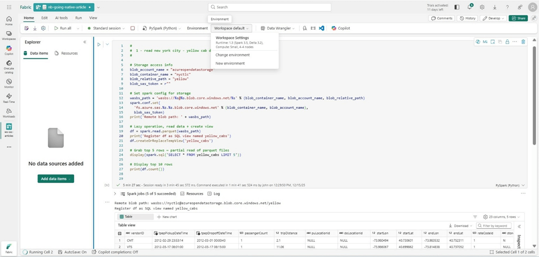
We need to have a sample program to tune. The following PySpark code has been identified as needing a faster execution time. We will focus on tuning this code using various techniques.
#
#  1 - New York City - yellow cab drivers dataset
#

# Storage access info
blob_account_name = "azureopendatastorage"
blob_container_name = "nyctlc"
blob_relative_path = "yellow"
blob_sas_token = r""

# Set spark config for storage
wasbs_path = 'wasbs://%s@%s.blob.core.windows.net/%s' % (blob_container_name, blob_account_name, blob_relative_path)
spark.conf.set(  'fs.azure.sas.%s.%s.blob.core.windows.net' % (blob_container_name, blob_account_name),  blob_sas_token )
print('Remote blob path: ' + wasbs_path)

# Lazy operation, read data + create view
df = spark.read.parquet(wasbs_path)
print('Register df as SQL view named yellow_cabs')
df.createOrReplaceTempView('yellow_cabs')

# Display top 10 rows
print(df.count())

# Grab top 5 rows ~ partial read of parquet files
display(spark.sql('SELECT * FROM yellow_cabs LIMIT 5'))
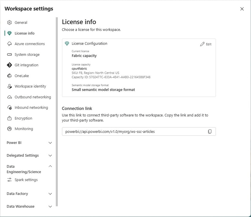
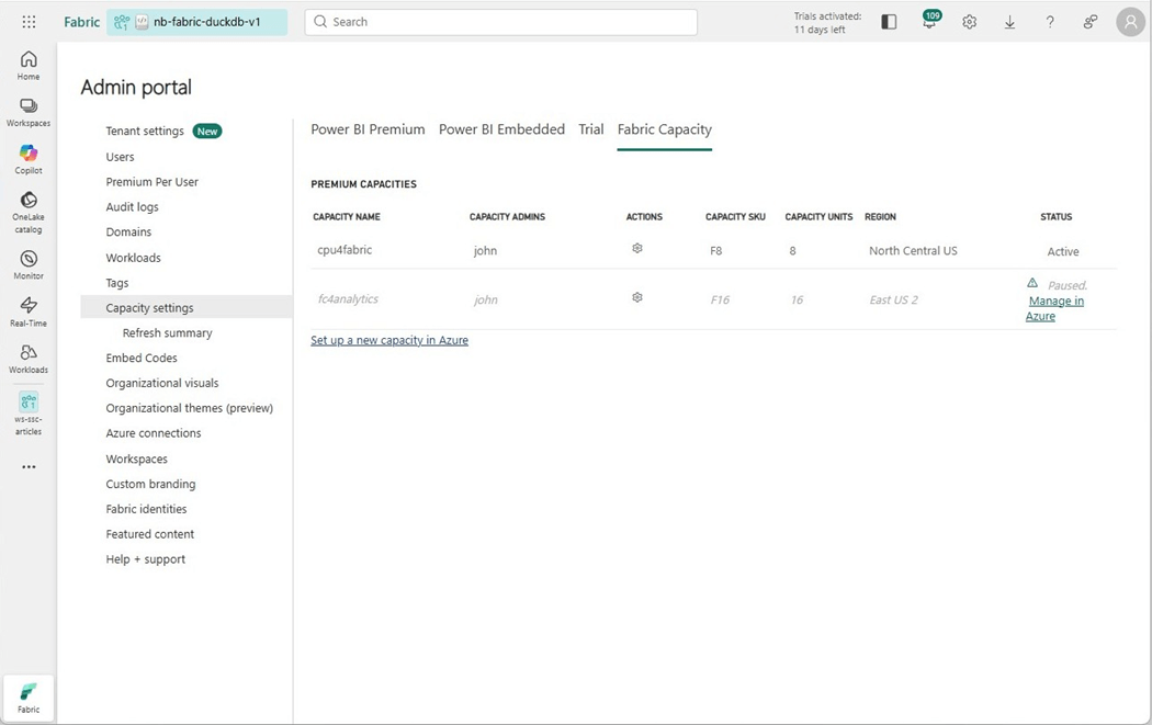
The capacity of the workspace is one limiting factor. We can see that an F8 SKU is being used in the image below. That means sixteen virtual cores can be used at most at one time.
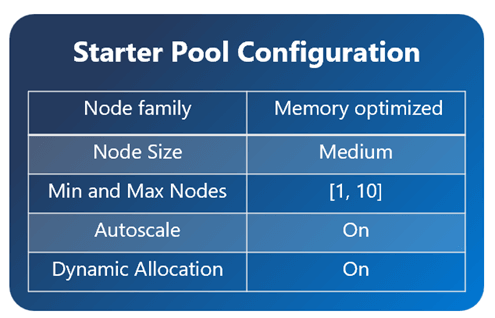
If we look at the default starter pool, the workspace settings below show that we can have up to six medium nodes.
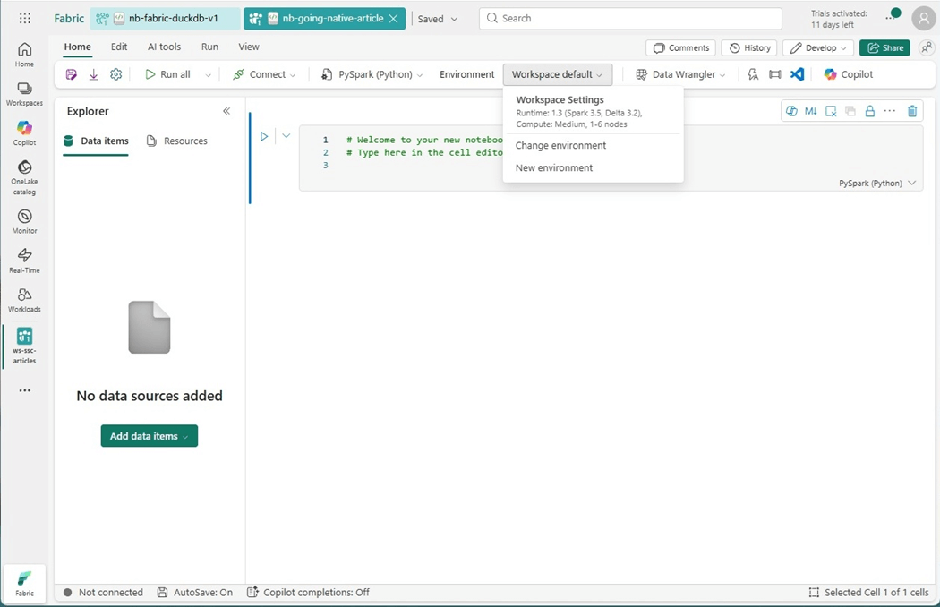
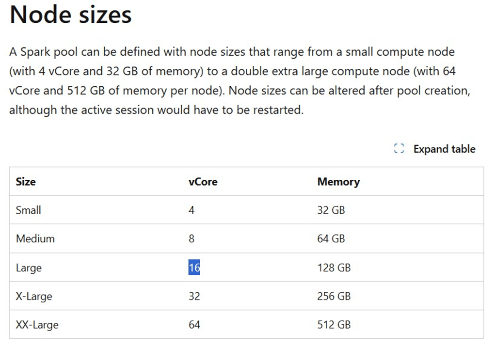
If we look up the nodes sizes, we can see a medium node has eight virtual cores. If we do simple math, the capacity has sixteen virtual cores, but the Spark Session says we can uses forty-eight total cores in a six-node cluster. How is this so?
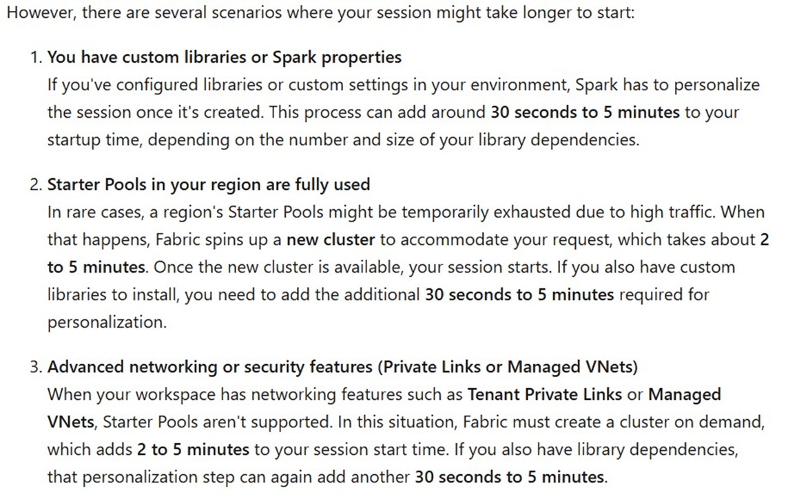
This is where the concepts of bursting and throttling come into play. Please see on line documentation for details. We can bust up to three times the capacity. However, there is no free lunch. We will be throttled in the future to pay back the temporary scaling in computing power. Please see the paragraph below for when starter pools might take a long time to start! Typically, a starter pool connects to a standard session in seconds.
I ran into this same issue with a client when an ODBC driver had to be installed as part of the environment. To recap, starter pools are impressive but there are some configurations that will take more time to start.
Standard Session with Bursting Enabled
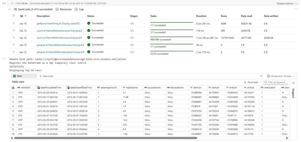
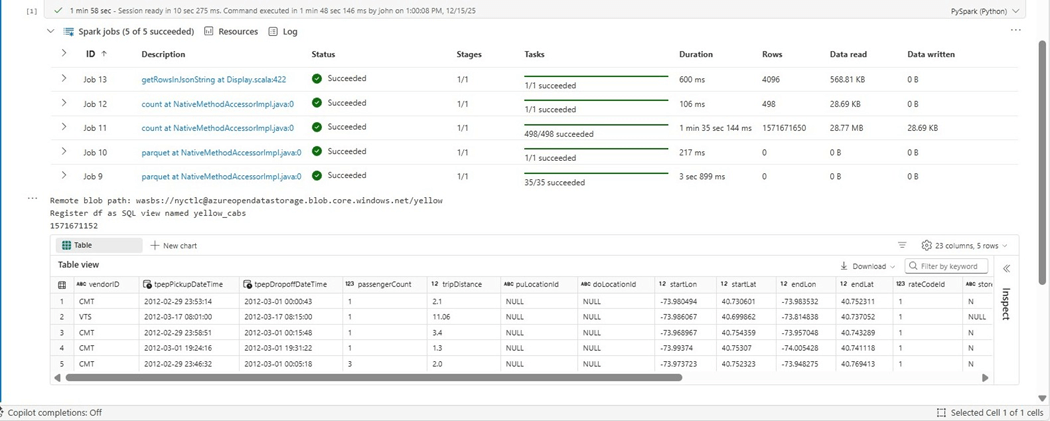
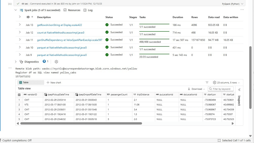
The image below shows the execution of PySpark code. If we did not have a count operation, we would just scan one random file and bring back ten records. Instead, we need to read each parquet file and get the record count. Job 15 shows it took almost five hundred rows or file counts to complete this task.
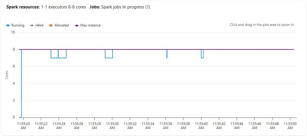
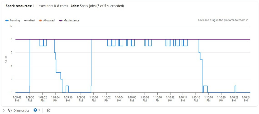
How many virtual cores did we use to accomplish these jobs?
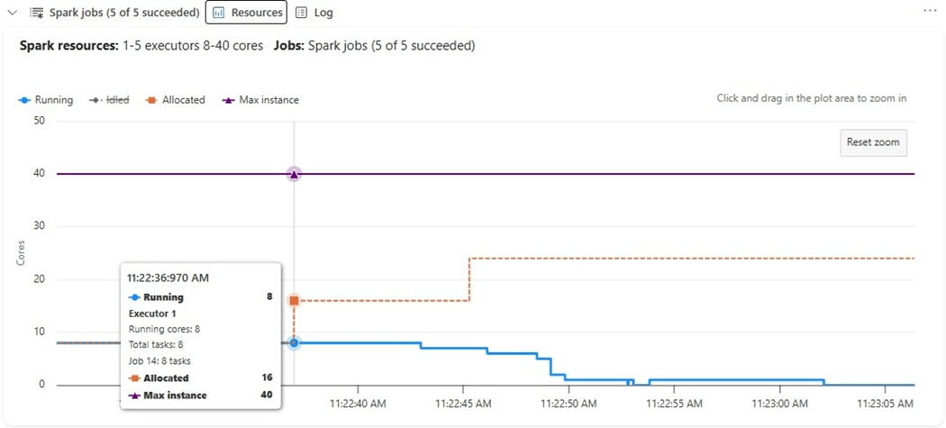

We can see that up to twenty-four cores were allocated to execute this distributed code but only eight were used (running). The graph is misleading since it shows a maximum of forty cores. The reason for this limit is that one node is the driver that controls the job execution and that medium size node takes eight virtual cores.
Be careful that you do not run out of capacity when running multiple notebooks.
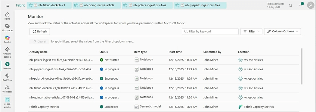
The above image of the monitor hub shows what is currently executing regardless of Fabric object type. We have five notebooks running. The sessions stay open until they time out. If you receive an out of capacity message when executing a cell, check the monitor for open and forgotten activities.
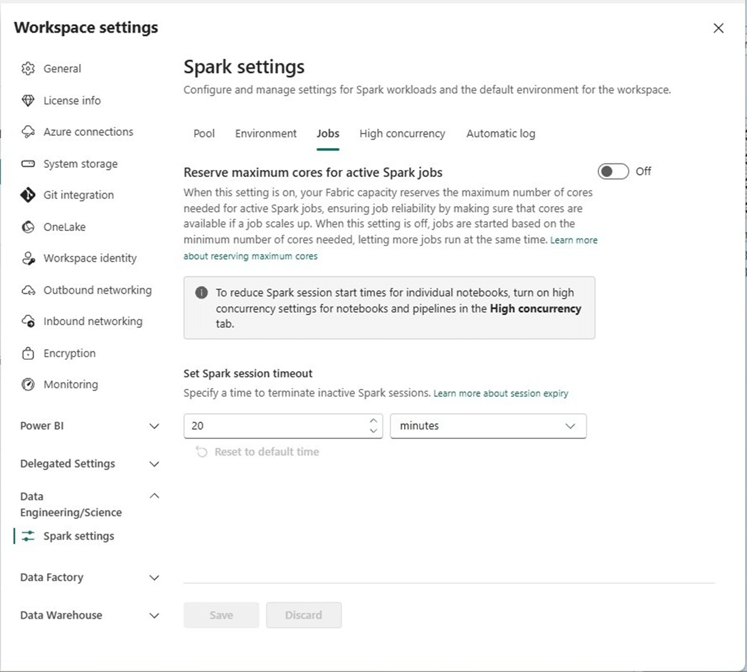
We can change the default Spark settings job timeout from twenty minutes to five minutes so that forgotten sessions are automatically closed. The above image shows the default setting on the jobs panel.
Standard Session with Bursting Disabled
The first task is to disable bursting. Please go into the admin portal and find the capacity settings page. Next, click the hyperlink of the capacity you want to configure.
Change the spark settings to not allow bursting. Please note, if we want to force everyone to use pools that we declare, we can disable the customized workspace pools and disable starter pools. This would require us to define pool for use by the end users. Please see documentation for details.
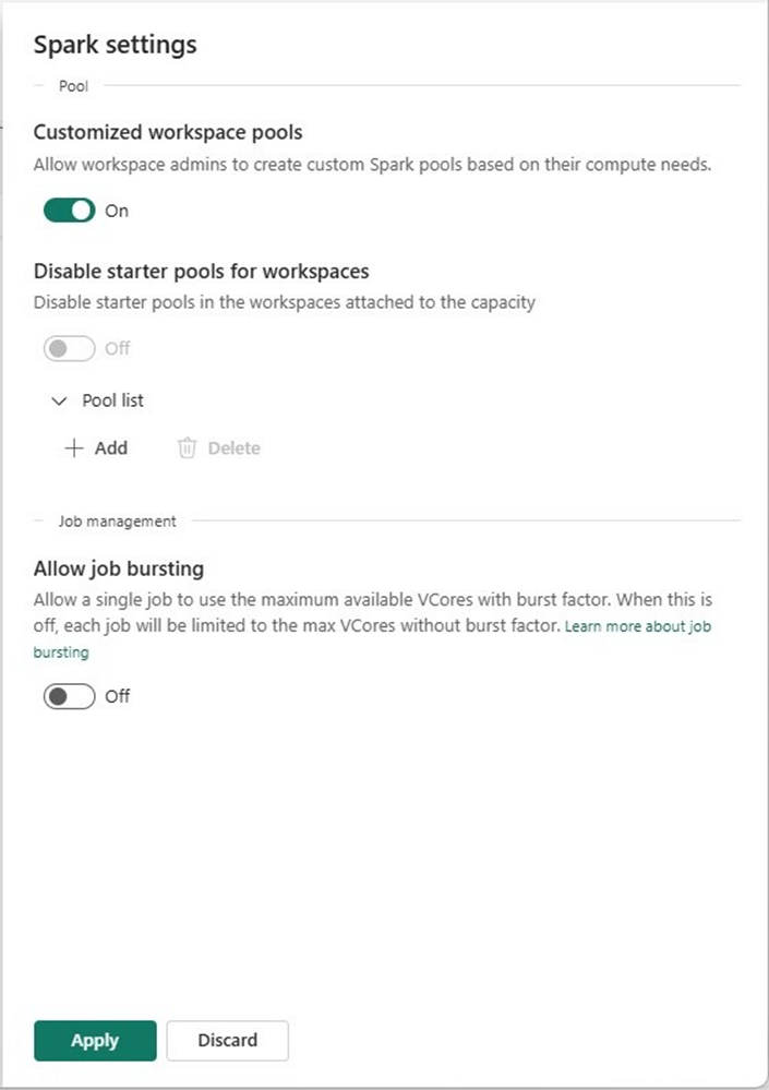
Make sure you apply the settings to complete the task. We can look at the workspace settings for data engineering and science. We can see that the tenant level change affected the workspace settings.
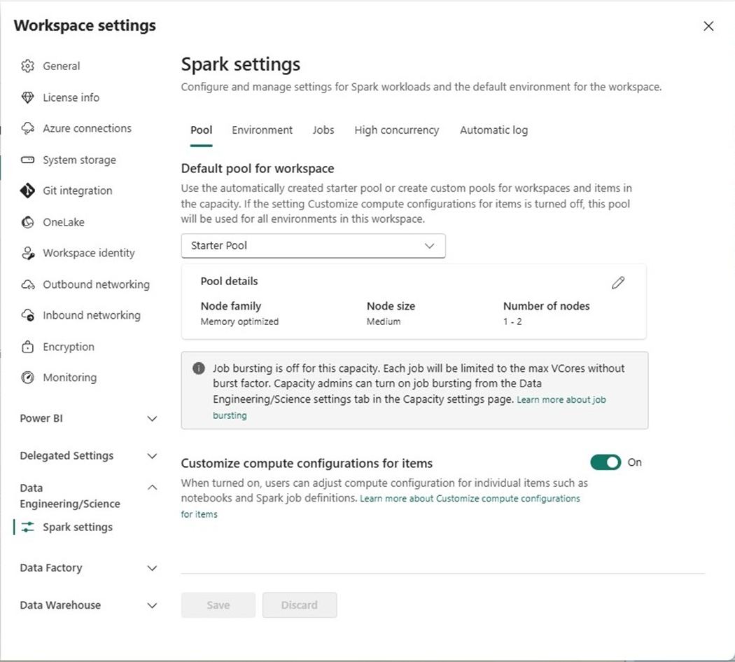
One major change we can identify without executing the program is the drop down for the default workspace settings. We can see only 1-2 nodes are available versus the 1-6 we had during the first execution.
There is only a few seconds difference between the two standard sessions. The bulk of the processing is reading in all the rows to get a correct count.
The graph of the executors is different. Since we have only eight virtual cores, we are fully using everything, and no scaling occurs with un-used but allocated cores.
Disabling bursting at the tenant level saved our boss money and did not decrease the total execution time.
High Concurrency Session
Lets take a look at two different sessions using the same starter pool (cluster). The image below shows the “going native” notebook.

The image below shows the “ingest csv files” notebook. They both share the same resources (Spark cluster).

The execution time remains the same. We are just sharing resources. Since I did not run them in parallel, there is no change.
Custom Pool Size
Another option that workspace owners have is the ability to create a custom spark pool size and set it as the workspace default.
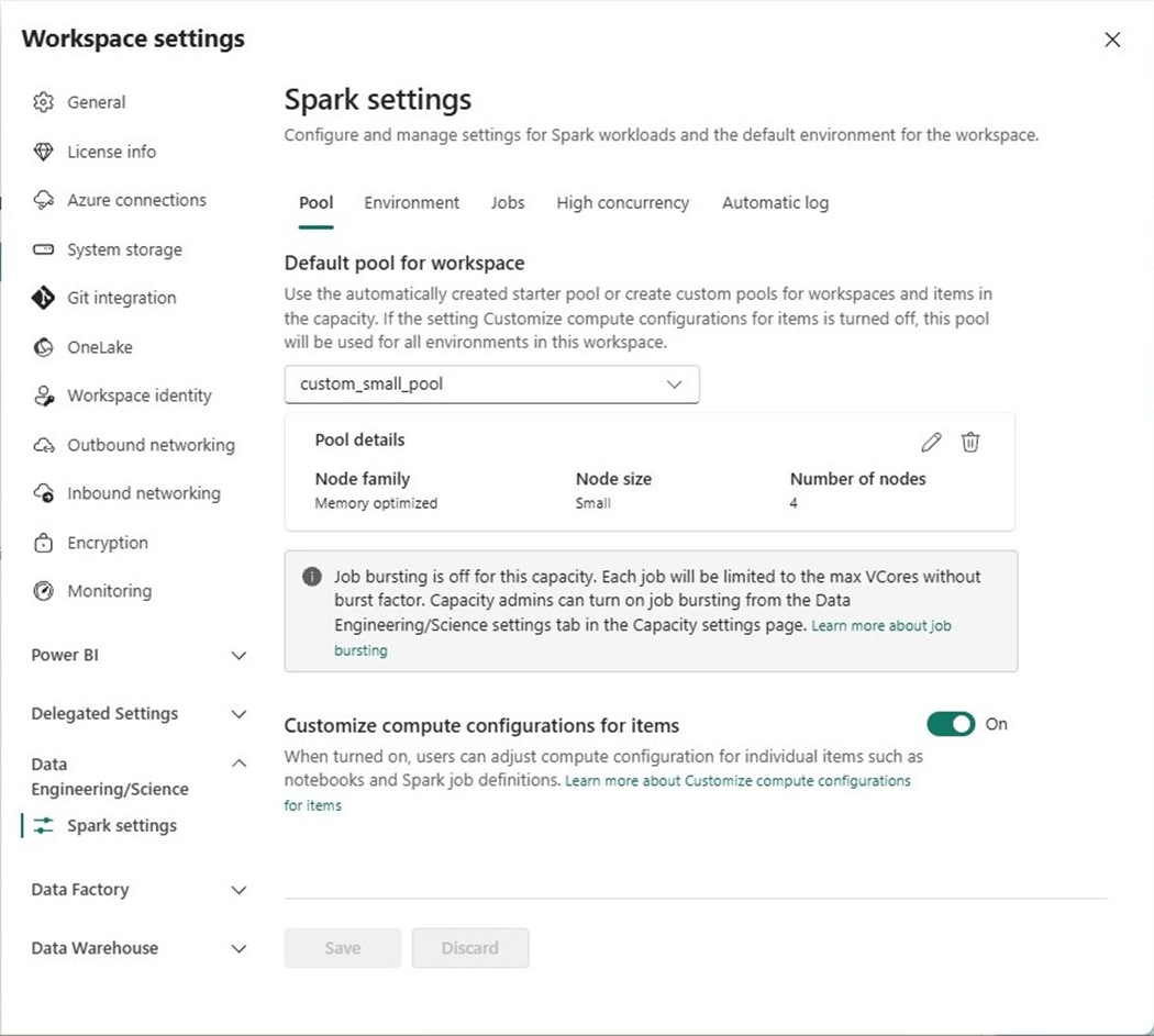
A capacity with an F8 SKU has sixteen cores. A small node size uses four cores. Therefore, we can have a four-node cluster. Let us see if this custom starter cluster executes the PySpark program any faster?
The execution time was shorter by 10 seconds. Moving the count operation to the bottom of the cell might be the culprit. However, the startup time was almost four minutes! Remember, starter clusters have to have a medium node size. Deviating from the starter requirements results in a custom cluster.
Native Execution Engine
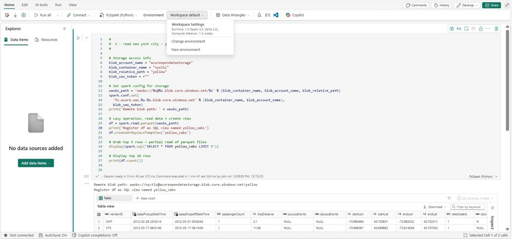
To leverage the native execution engine, we must create an environment. We can do this by hitting the new item (+) on the workspace and search for the “environment” key word.
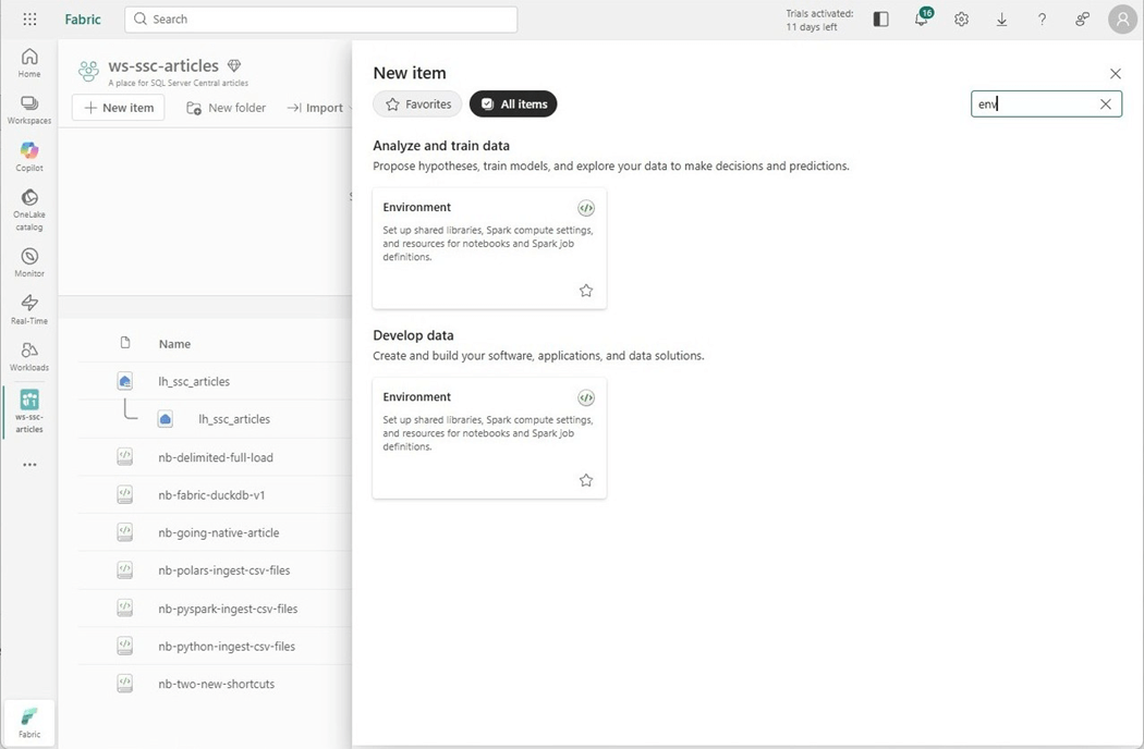
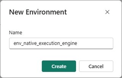
Of course, we have to give the environment a name.
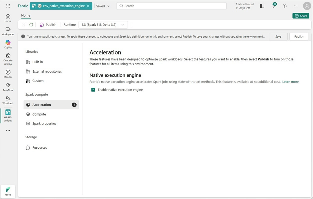
Typically, environments were used to load custom libraries, set computing configurations and/or apply spark settings. Any of these changes does not allow the Spark session to use a starter pool. However, if we just enable the native execution engine for acceleration, we can use the default starter pool.
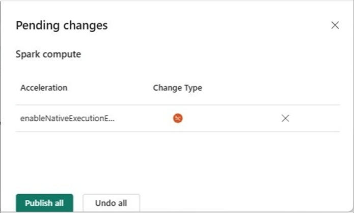
We need to publish the environment before we can choose it in our PySpark notebook.
The image below shows the environment that has been selected. Click execute cell arrow to start the job.
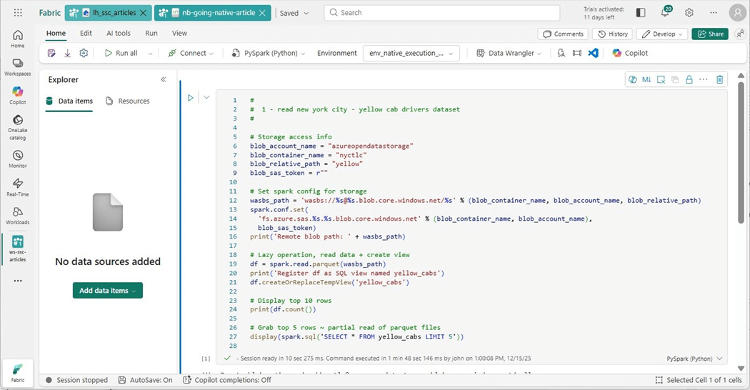
The job that reads the 1.5 Billon rows now takes 17 seconds. It typically took around one hundred seconds to execute. That means the native execution engine is five hundred percent faster.
The spark resources show a different pattern than the previous executions. We have a choppy graph instead of a step function or sloping graph.
Experimental Findings
Today, we tried five different spark configurations while executing the same PySpark program. The first three configurations have the same execution time. Because the custom pool could not use a starter pool, the execution time was over 5 minutes due to cluster startup. The environment with the native execution engine was the clear winner.
| Configuration | Execution Time (s) | Max v-Cores
| Comments
|
| 1 | 116 | 24 | Standard session with bursting enabled |
| 2 | 118 | 16 | Standard session with bursting enabled |
| 3 | 118 | 8 | High concurrency session with bursting disabled |
| 4 | 327 | 8 | Custom pool with four small nodes |
| 5 | 44 | 8 | Native execution engine using standard session. |
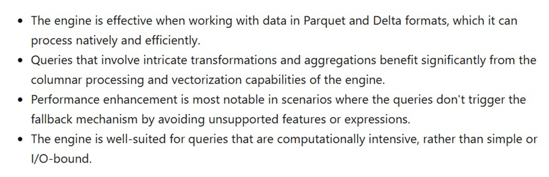
The image below is a paragraph taken from the MS learn website. I chose to work with Parquet files since I knew the engine would read them quicker than the Scala JVM engine. If I chose to work with CSV files, the engine would have fallen back to the standard JVM engine. Any computational and/or intricate transformations will benefit from the new native execution engine.
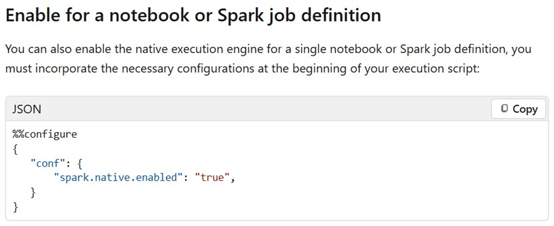
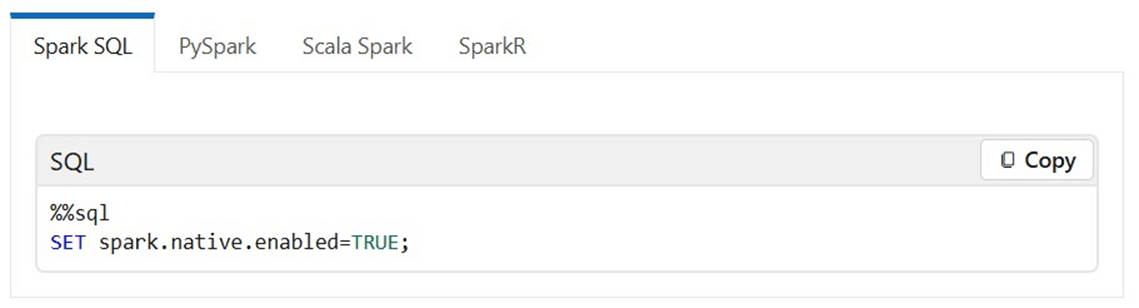
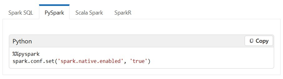
The paragraph below was taken from the MS learn website. We can turn on or off the engine at both the notebook and cell levels. The code below configures the whole notebook to try to use the new engine.
We can enable or disable the engine for Spark SQL at the cell level.
Of course, we can do the same for PySpark.
There are a bunch of limitations and cautions that you should read before switching to the new engine. Please see documentation for details. To recap, the native execution engine had the best runtime using the least amount of resources.
Summary
As a Fabric data engineer, it is important to understand where changes can be made for Data Engineering using Spark. The tenant level settings can be used to disable or enable starter pools. Additionally, we can disable bursting. Just remember, there is a queue length and retry logic that should be used in the data pipeline. We can also force end users to use pools that administrators set up at the tenant level. Just remember starter pools allow one to ten medium size nodes. After that limit is exceeded, a normal spark cluster start time is two to five minutes.
The workspace settings allow administrators to create environments and custom pools. Again, not using medium size nodes will result in a longer startup time. On the other hand, if you are using high concurrency sessions, an extra-large cluster can be shared between multiple people. Standard sessions use resources but can not be shared between notebooks and/or users. One of the most important workspace settings is the cluster timeout. Too short of a time results in restarting a session. Too long of a time might result in an out-of-resource situation. One can use an environment to apply custom libraries, spark settings, and/or drivers. Just remember these environments cannot use a starter pool.
Finally, the native execution engine shows tremendous speed improvement with reading parquet and delta files. We can control the use of native execute engines for notebooks via custom environments, notebook configurations, and/or cell settings. One thing I leave the reader to explore is the use of the engine with complex calculations. Here is a summary of limitations that you might encounter: date filter type mismatches, decimal to float casting issues, inconsistent rounding behavior, time zone configuration error handling, skipping duplicate key check in mapping function, no support for UDFs, no support for text related formats, and order variance / type mismatch for collect functions. Please see the limitations section of on-line documentation for complete details.
In short, the native execution engine is pretty amazing. It speeds up ingestion with the Velox enhancement and pushes JVM execution to natively compiled engine using Gluten. For standard Spark processing that has an enormous amount of parquet files or complex processing, one might want to look at this engine to decrease the time your data engineering pipeline runs with the same amount of resources.