Exploring DiskANN: Part I: Understanding the Algorithm before the disk
Mala Mahadevan, 2026-09-09 (first published: 2026-08-27)
How I used AI for this post
ChatGPT to generate images based on info specifically provided by me,including examples.
Grammarly to catch grammar and sentence construction errors.
I did a presentation on Vector Economics at EightKB, a popular SQL Server Internals conference, recently. The talk was well received. Among the follow up suggestions, one was about doing a blog series on DiskANN Algorithm – the algorithm created by Microsoft Research, documented here, and is used for vector index on SQL Server Vector Search.
DiskANN is meant to help with searching a billion-vector dataset from a single machine using SSDs.
Microsoft Research’s original work demonstrated a billion-point index on a workstation with 64 GB of RAM and an SSD, while targeting high recall and low query latency. Before we get to ‘why ssd’ and details of storage, we need to understand the basics of vector search and underlying terminologies.
Basics of Vector Search
Imagine we’re building semantic search for an online store. Our catalog contains below products:
P1 “Men’s waterproof hiking boots”
P2 “Women’s trail running shoes”
P3 “Insulated winter snow boots”
P4 “Lightweight camping tent”
P5 “Waterproof hiking backpack”
P6 “Running socks”
Assume that a customer is searching for: “boots for hiking in the rain”.
Full-text search can efficiently find and rank documents containing terms such as boots, hiking, and rain, while features such as stemming and fuzzy matching can handle variations of those words.
But what if the query says “boots for hiking in the rain” while the product description says “waterproof outdoor footwear”? There may be little direct word or phonetic overlap, even though the two clearly mean similar things.
This is where vector search is useful: instead of asking whether the words match, it gives us a way to search based on how closely their meaning is represented.
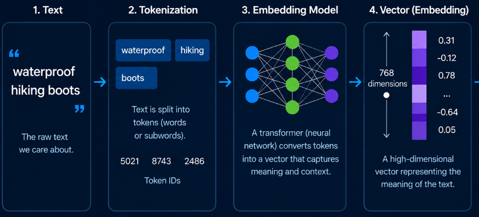
An embedding model converts each product into a vector:
“Men’s waterproof hiking boots” ->
[0.12, -0.73, 0.41, 0.08, …]
The customer’s query goes through the same process:
“boots for hiking in the rain” ->
[0.15, -0.69, 0.45, 0.04, …]
Then, these two vectors are compared. (There are multiple metrics one can use for comparison).
The closer the results are mathematically, the similar they are in semantic meaning. That is essentially how vector search works.
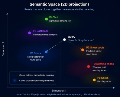
Each vector might contain hundreds or thousands of dimensions. Each individual number means nothing in of itself. Objects with similar meaning tend to occupy nearby regions of this high-dimensional space.
Illustrative 2-D projection of what is actually a high-dimensional vector space. (It is several hundred, or thousand dimensions)
The vector-search problem can be stated as:
“Given a query vector, find the vectors closest to it.”
Why do we need an index?
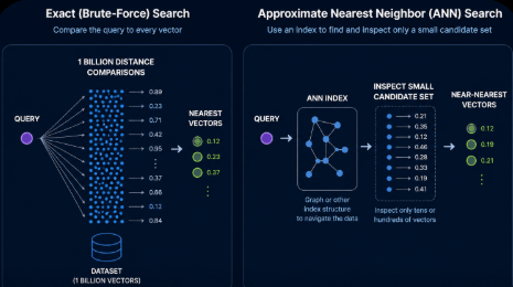
With a small list of six products, the obvious solution works perfectly. Compare the query against every product:
distance(query, P1)
distance(query, P2)
distance(query, P3)
distance(query, P4)
distance(query, P5)
distance(query, P6)
Then, sort the distances and return the nearest products. This is exact nearest-neighbor search. For a small number of vectors, we can scan every vector we have for comparison. But, But suppose our system contains a billion vectors. Or more.Every query potentially needs to be compared against a billion other vectors or more. This can get really expensive and time consuming. An ANN index tries to answer a different question:
Can we inspect only a small fraction of the billion vectors and find NEARLY all of the nearest ones?
ANN stands for ‘Approximate Nearest Neighbor’. The algorithm intentionally trades a small amount of certainty for a potentially enormous reduction in search work.
Before looking at how DiskANN accomplishes that, let us try to understand the vocabulary around it.
DiskANN vocabulary
Vector / Point / Node
A vector in general , is simply an ordered list of numbers – like below.
[0.12, -0.73, 0.41, 0.08, …]
An embedding is a vector with a particular purpose—produced by a model to represent something, such as text, an image, or a product, in a numerical space where similarity can be measured. Every embedding is a vector, but not every vector is an embedding. In this context, we are talking about vectors as they represent embeddings. Every embedding is a vector, but not every vector is an embedding. In this context we are talking of vectors as they represent embeddings.
Once that vector becomes part of a graph, we can think of it as a node or vertex. In the context of DiskANN we can consider them equivalent terms.
Distance
We need a way to answer: How similar is this vector to my query?
Similarity can generally be measured using 3 metrics. They are cosine, Euclidean, and dot product. More details can be found here. We will use cosine for this demo. With that metric, the smaller the distance, the more similar the vector is to the query vector.
Neighbor
If two vectors are close in embedding space, we can treat them as neighbors. For example, hiking boots may be ‘close’ to ‘Rain boots’ or ‘Snow boots’.DiskANN’s graph stores selected relationships like these as edges. “Neighbor” does not simply mean “the closest vector.” That distinction is important.
Graph
A stored connection between two vector nodes that gives graph search a route from one vector to another. Vector distances help determine which edges should exist, but DiskANN does not simply connect every vector to its nearest neighbors—it selectively keeps edges that help make the graph navigable.The graph becomes a map that search can navigate.
Degree
The degree of a node is, roughly speaking, how many graph connections it has. Degrees matter because connecting every node to everything else would defeat the purpose.
DiskANN wants a graph with a limited number of useful edges. But, how does it determine which edges deserve to exist? We’ll answer that when we get to the pruning strategy.
Entry point / Medoid
Graph search needs to begin at any one node. One strategy represented in the DiskANN code is starting from a medoid—roughly, a representative central point of the dataset.
It gives search a reasonable place from which to begin navigating.
Greedy graph traversal
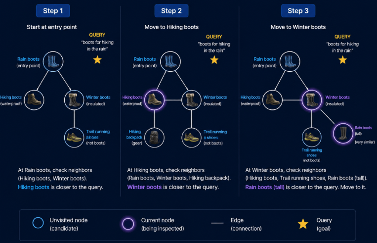
Once our vectors have been organized into a graph, we need a way to search it. One key idea behind DiskANN is ‘greedy graph traversal‘.
At each step, the search looks at the neighbors available from its current node and prioritizes the one that appears closest to the query vector.Consider our query: “boots for hiking in the rain”. A simplified traversal would be –
Step 1 — Start at the entry point.
Suppose the search starts at a node called ‘Rain boots’. Ot examines the nodes connected to ‘Rain boots’. Of the available candidates, ‘Hiking boots’ is closer to our query, so the search moves in that direction.
Step 2 — Explore the new neighborhood.
From ‘Hiking boots’, the search discovers another set of neighbors. It compares those candidates with the query and finds ‘Winter boots‘ promising, so the traversal continues there.
Step 3 — Keep moving toward the query.
From ‘Winter boots’, another ‘Rain boots’ type of vector becomes visible. Its embedding is even closer to the query, so it becomes the next candidate.
The graph behaves like a map through the vector space.The edges tell the search which vectors are worth considering next, and vector distance tells it which of those candidates looks most promising. This is a simplified example. Real DiskANN search doesn’t blindly follow a single path and forget everything else. It maintains a candidate list of promising nodes so it can return to another route if necessary. That distinction leads to the next DiskANN concept: the search list, or L.
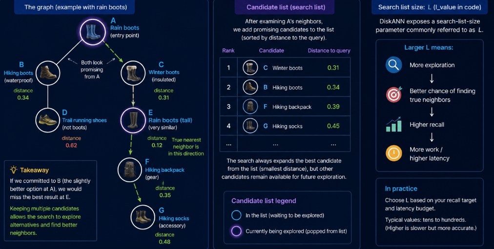
Candidate list / Search list (L)
Committing to a single path is risky. Looking at the search term in our example –
“boots for hiking in the rain”
Suppose the search begins at ‘Rain boots’. From there, it discovers two promising neighbors: ‘Hiking boots‘ and ‘Winter boots’. Both look relevant. One may appear slightly more promising than the other, but we don’t yet know what lies beyond them in the graph. The best result might be several hops away through either route. If we choose one path and permanently discard the other, we could miss a much better result.
This is why graph-based ANN search maintains a ‘candidate list’, sometimes called the ‘search list’ or ‘frontier’. As promising nodes are discovered, they’re added to this list and ordered according to their distance from the query.DiskANN controls the size of this search list using a parameter commonly called L (l_value in the implementation). L controls how much of the graph search the algorithm is willing to explore. A small L keeps fewer possibilities alive. It is faster, but increases the chance that a useful route is discarded. A larger L allows the search to consider more candidates. This is one of the fundamental ANN tradeoffs.
Recall
ANN search is approximate. We need to measure how often it finds the answers an exact search would have found.Suppose our query is:
“boots for hiking in the rain”
If we perform an ‘exact search’ over the entire catalog, imagine the true 5 nearest products are:
1. Waterproof hiking boots
2. Tall rain boots
3. Lightweight rain boots
4. Insulated waterproof boots
5. Waterproof trail shoes
Now suppose DiskANN’s approximate search returns:
1. Waterproof hiking boots ?
2. Tall rain boots ?
3. Lightweight rain boots ?
4. Waterproof trail shoes ?
5. Hiking shoes ?
DiskANN found 4 of the true top 5 results. So, Recall@5=54?=80% (for this one query, not the entire dataset). High recall means our approximate search behaves more like exact search.
Beam width
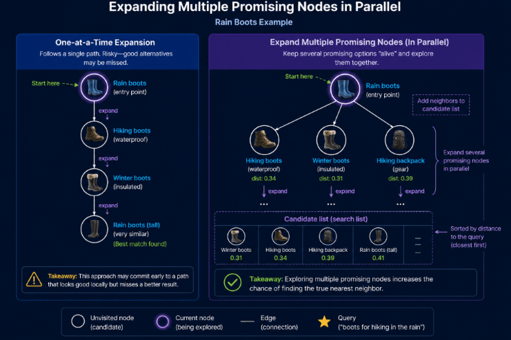
We’ve seen that DiskANN keeps a ‘candidate list‘ rather than committing permanently to one path. There is more to it: instead of expanding candidates strictly one at a time, search can expand several promising nodes together. Return to our query:
“boots for hiking in the rain”
Starting from Rain boots, the graph might expose several promising neighbors – such as ‘winter boots’ , ‘hiking boots’, or even a ‘hiking backpack’. Think of beam width as:
How many promising graph nodes can we expand simultaneously?
Its importance becomes much clearer when DiskANN starts fetching graph data from SSD.
RobustPrune , Alpha and R
These terms belong primarily to building the graph rather than searching it.
RobustPrune is a procedure for deciding which candidate edges are worth keeping.
Alpha is a parameter that determines how aggressively candidate neighbors are considered redundant during pruning.
Ris a Vamana/DiskANN index-build parameter that controls the maximum degree of the graph—the ‘edge budget’, or roughly how many outgoing edges each node is allowed to keep after pruning.
From Vector Search to Graph Search
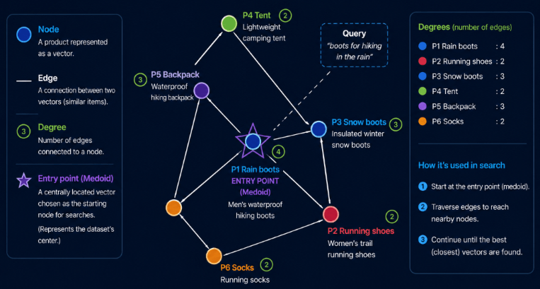
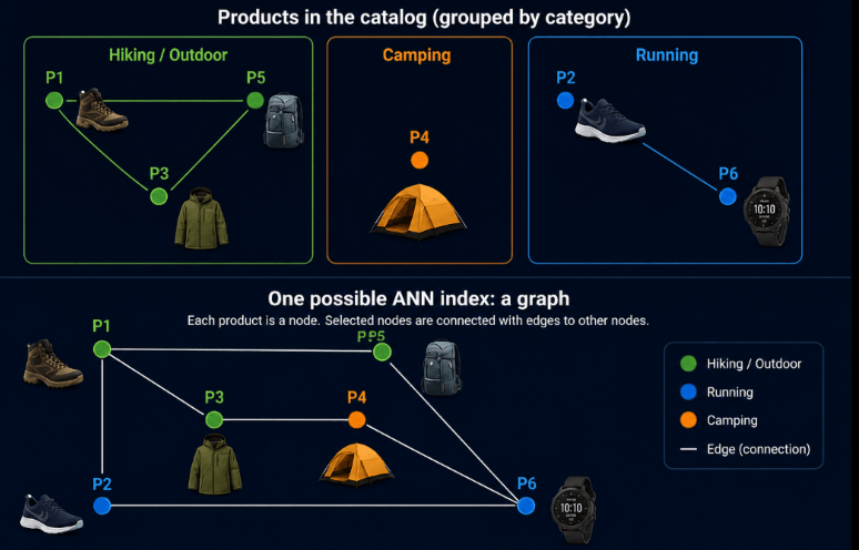
Let’s return to our product catalog.Imagine how products are grouped by rough categories, as below.
A query no longer needs to inspect every product. Instead, it can navigate the graph. This changes vector search from ‘Compare the query against everything’ to ‘Start somewhere reasonable and use the graph to discover increasingly promising candidates.’ That’s the fundamental abstraction behind graph-based ANN. That leads to how nodes/vectors are connected.
Why not simply connect every vector to its nearest neighbors?
At first, building the graph seems straightforward: for every vector, find its closest vectors and connect them.
Consider node A — ‘Rain boots’. Suppose its four closest vectors are B, C, D and E, all representing very similar rain boots. Connecting A to all four seems sensible—they are, after all, its nearest neighbors.
But there’s a problem: B, C, D and E may all occupy essentially the same small region of the vector space.
A has what we can call an ‘edge budget’ (R) – limited number of edges. Using nearly all of them to connect to very similar vectors gives us excellent knowledge of A’s immediate neighborhood, but those connections are somewhat redundant. If search reaches A, every available route may take it to roughly the same place. In other words, it may not matter to a purchaser of Rain boots if they get to A, and then B, C, D or E..they are all very close as products. The results are not hugely diverse.
Now consider X — Tall rain boots and Y — Green rain boots. They aren’t as close to A as B, C, D and E are, but they represent different regions of the vector space. In other words, the product is a bit different, in an interesting way. The purchaser may suddenly decide, hey, ‘tall boots’ , maybe I do need some of those, not just this ‘rain boot’ with a regular length. Using some of A’s limited edge budget to create routes toward those (more diverse) regions can make the graph much easier to navigate (and the results more interesting). But it is also a bit of a design problem.
Given a limited number of edges per node, how do we choose a set of neighbors that makes the entire graph easy to navigate and result in a diverse result set?
Meet Vamana
Microsoft Research introduced ‘Vamana‘ as part of the original DiskANN system, describing it as a new graph-based ANNs index that was useful even independently as an in-memory graph index. Vamana constructs the graph that DiskANN will eventually search.
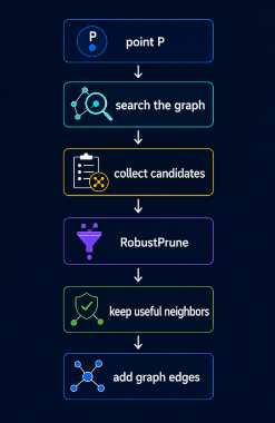
The high-level looping structure may be as follows.
Let us examine those steps in more detail.
Building one node’s neighborhood
Point P – Search the Graph – Collect Candidates
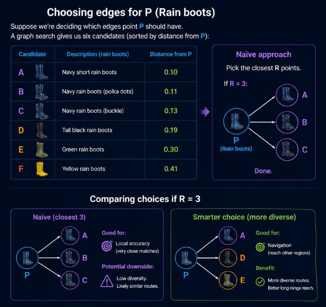
Suppose we’re deciding which edges P — ‘Rain boots’ should have. I have an ‘edge budget'(R) of 3. Why do I even need an ‘edge budget’? Because not every node can connect to every other node; we are limited in resources. A graph search has already given us six candidate neighbors, ordered by their distance from P.
A Navy short rain boots 0.10
B Navy rain boots 0.11
C Navy rain boots 0.13
D Tall black rain boots 0.19
E Green rain boots 0.30
F Yellow rain boots 0.41
If P is allowed a maximum of three edges (R = 3), the obvious strategy would be to simply choose the three closest candidates:
P ? A
P ? B
P ? C
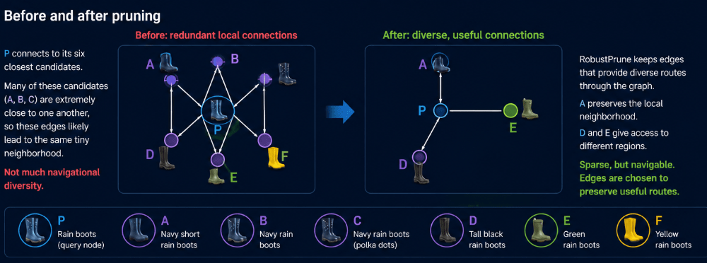
That gives P excellent connections to its immediate neighborhood. But look at the geometry in the diagram: A, B and C are also extremely close to one another (A and B are separated by 0.01 and B and C by 0.03). Once P has an edge to A, adding edges to B and C doesn’t give me any additional value. All 3 connections potentially lead search into essentially the same part of the vector space. We’ve used our entire three-edge budget, but haven’t created much diversity in where those edges can take us.
RobustPrune: Keep useful neighbors
The RobustPrune procedure evaluates candidates and poses the question:
“If I’ve already selected this neighbor, does another candidate still give me a sufficiently useful connection?”
It gives Vamana a systematic way to ask:
“If I’ve already kept A, do I really need a direct edge to B—or does A already give me a good enough route toward B’s neighborhood?“
If B is effectively redundant, it can be pruned, leaving room in P’s limited edge budget for a candidate that adds more navigational value.
RobustPrune considers the relationships between the candidates themselves, not just their individual distances from P.
Instead, imagine keeping A but also retaining D and E.
P ? A close local neighbor
P ? D another useful direction
P ? E access to another region
D and E are farther from P than B and C, but that doesn’t automatically make them worse graph neighbors. They may provide routes into portions of the graph that aren’t already easily reachable through A.
This illustrates an important distinction:
Distance alone tells us which vectors are similar. Graph construction has to decide which connections are useful for navigation – in order to find the best matches in the shortest time.
The goal therefore isn’t simply to minimize the distance of every edge. It’s to build a small set of edges that collectively gives search useful routes through the vector space.This is where RobustPrune adds value.
The resulting graph is sparse, but its edges are deliberately chosen to preserve useful routes. This is a much deeper and better idea than simply “connect every vector to its nearest neighbors.”
Where ‘alpha’ fits
The current repository configuration uses 1.2 as a default alpha in its graph-index configuration. What is ‘alpha’ ? Alpha influences when RobustPrune decides:
“I’ve already selected a neighbor that makes this candidate sufficiently redundant.” In other words, it is how aggressively RobustPrune decides that one neighbor makes another neighbor redundant.
Suppose we’re pruning the outgoing edges for our P = Rain boots node. We have these candidate neighbors:
P = Rain boots
A = Navy rain boots
B = Waterproof hiking boots
C = Tall rain boots
D = Winter boots
E = Green rain boots
Robust prune picks the first possible candidate, A , and connects it to P.
Suppose d stands for distance and d(P,B) = 0.3 while d(A,B) = 0.2 .
Alpha (simplified) is checking if d(A,B) <= d(P,B).
With Alpha = 1.0, If we check if 1.0 x 0.20 <= 0.30, yes it is. So RobustPrune can essentially say: “A is already close enough to B. I don’t necessarily need P->B.” Then it proceeds to prune/remove P->B.
With Alpha = 1.5, the test is if 1.5×0.20 <= 0.30. This is still true, so the decision with 1 to prune P->B is still valid.
With Alpha = 2.0, the test becomes 2.0×2.0<=0.30. Now this is false. Now B survives this pruning test.
Increasing alpha generally makes the pruning condition harder to satisfy, so fewer candidates are eliminated as redundant by a selected neighbor.Higher alpha makes RobustPrune less willing to eliminate a candidate because another selected neighbor is nearby, changing which edges survive within the R-edge budget.
Summary
Summarizing the terms learned –
Term
Simple meaning
Vector
the numerical representation of an item
Distance
how similar or dissimilar two vectors are
Node
a vector represented as a point in the graph
Graph
the map we navigate
Edge
a route we are allowed to explore
Degree
how many edges a node has
Medoid
a centrally located node used as a starting point for navigation
Candidate
a node we’re considering as potentially useful
Candidate list / frontier
promising nodes we haven’t finished exploring
Greedy traversal
prioritize candidates that currently look closer to the query
ANN
find very close neighbors without checking every vector
Recall
how often we recover the true nearest neighbors
Terminologies relevant to graph building/pruning may be –
Term
Simple meaning
RobustPrune
remove redundant edges while preserving useful routes
R
the maximum number of outgoing edges a node is allowed to retain
a (alpha)
how strong the evidence must be before one candidate makes another candidate redundant
Redundant edge
an edge we may not need because another neighbor already provides a good route there
Edge budget
an intuitive way to think about the limited number of connections available under R
Neighbor diversity
keeping edges that provide meaningfully different routes through the graph
Pruning
deciding which candidate edges to discard
Reverse edge
a connection added back from a selected neighbor toward the node during graph construction
Ok, so where is the “Disk” in DiskANN?
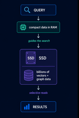
Graph search works well when the graph and vector data fit comfortably in memory. But at high volume (billions of vectors), keeping everything in RAM becomes expensive and impractical.
This is where the “Disk” in DiskANN becomes relevant .
DiskANN was designed around keeping a compact representation of the index in memory, while placing the much larger graph and full-precision vector data on SSD. The graph’s navigability helps search avoid random access across the entire dataset—it only needs to fetch a relatively small number of promising nodes from SSD. That combination allowed DiskANN to demonstrate high-recall, low-latency ANN search over datasets much larger than available memory.
But making graph traversal work efficiently when its data lives on SSD introduces an entirely new set of engineering problems: what stays in RAM, what goes to disk, how many SSD reads a query requires, and how those reads are scheduled.
That’s where we’ll pick up in Part 2: taking DiskANN from memory to disk.
Next: Part 2: Putting the “Disk” in DiskANN — PQ, SSDs, caching and beam search.