DiskANN Experiment — Exploring Entry Points and Graph Neighborhoods
Mala Mahadevan, 2026-10-26 (first published: 2026-10-19)
Introduction
I was experimenting with vector search in SQL Server 2025 using approximately 3.8 million Hacker News articles that that I used for my talk on SQL Server-based vector search feature at EightKB. I generated two sets of embeddings from the same articles: one stored as FP32 (32-bit floating point) and the other as FP16 (16-bit floating point). Both sets contained the same articles and used DiskANN vector indexes.I used a query as below to find articles similar to a selected example.
DECLARE @QueryVector VECTOR(768, FLOAT32);
-- Get the embedding of our example article.
SELECT @QueryVector = embedding
FROM dbo.ArticlesEmbeddings_FP32
WHERE hn_id =18349232;
-- Find the 10 most similar articles.
SELECT TOP (10)
e.hn_id,
vs.distance
FROM VECTOR_SEARCH(
TABLE= dbo.ArticlesEmbeddings_FP32 AS e,
COLUMN= embedding,
SIMILAR_TO = @QueryVector,
METRIC ='cosine',
TOP_N =11
)AS vs
WHERE e.hn_id <>18349232
ORDERBY vs.distance;
The query takes the embedding of one article and uses SQL Server’s vector index to find articles with similar embeddings. The distance value tells us how close the articles are: a smaller cosine distance means greater similarity.I then ran the equivalent query against the FP16 table, using an FP16 query vector. I expected FP16 to be faster, or at least require fewer logical reads. After all, an FP16 embedding uses roughly half the storage of an FP32 embedding.But that wasn’t always the case. Some FP16 searches were slower and performed more logical reads than the equivalent FP32 searches, although the size of embeddings were half the size of FP32.It made me wonder whether the difference had less to do with embedding size and more to do with how SQL Server builds and searches its DiskANN vector indexes.There are two possible explanations:
1. SQL Server’s FP32 and FP16 indexes report different starting nodes, based on the sys.vector_indexes DMV. Even if the graphs are nearly identical, beginning in different places could lead the search through different parts of the graph and require different amounts of work.
2. Although the graphs are similar, they are not identical. A few different connections could cause the search to discover different articles, follow different routes, and perform more or fewer comparisons.
I engaged in two experiments for this purpose.
Experiment A — Graph structure and ranking
Determine whether changing vector precision from FP32 to FP16 changes the reconstructed graph’s connections or the ranking of candidates.
Experiment B — Search traversal
Determine whether the small differences between the FP32 and FP16 reconstructed graphs cause the search to perform different amounts of work, and whether the different starting points contribute to those differences.
In this blog post, I’ll explore Experiment A. These experiments are only exploratory recreations of the DiskANN algorithm, based on what we know of its parameters, using SQL Server Graph tables. They are not a replica of the index.
As a first step, I tried to recreate DiskANN’s graph structure using SQL Server Graph tables. DiskANN algorithm has many parameters. Not all of them are exposed in the SQL Server implementation. You can view what is exposed in the build_parameters column using the query below.
SELECT
i.name,
vi.vector_index_type as index,
vi.distance_metric,
vi.build_parameters
FROM sys.vector_indexes AS vi
JOIN sys.indexes AS i
ON i.object_id = vi.object_id
AND i.index_id = vi.index_id;
My results for my FP32 and FP16 indexes are below.
Microsoft has marked the build_parameters column as ‘for internal use only’. We don’t know how these parameters are used. But based on the algorithm, we can reasonably assume L stands for Search List/Candidate List Size, and R stands for the maximum degree of the graph index. It is unclear what M means.
To construct the simulated graph, I used the parameters reported by SQL Server’s DiskANN indexes as a starting point.
I treated R = 48 as the maximum number of outgoing connections each node could have.
I used L = 48 as the search-list size when exploring the graph, but not as a limit on the number of connections.
For graph construction, I considered up to 192 candidate neighbors (4×R) for each node, then selected the best connections using cosine distance and a pruning factor of 1.2 to avoid keeping too many similar neighbors.
I also allowed reverse-edge proposals to help connect the graph.
StartID seemed to align with hn_id, the key defined in the embedding tables, so I used that.
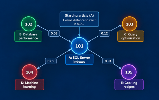
Imagine we have five rows in our embeddings table. Each row represents a Hacker News article and contains a 768-dimensional vector describing its content.
embedding_id
Article
Example cosine distance from A
101
A: SQL Server indexes
0.00
102
B: Database performance
0.08
103
C: Query optimization
0.12
104
D: Machine learning
0.65
105
E: Cooking recipes
0.91
Illustrative graph built from those rows may look as below.
The graph-building process works as follows:
1. Create nodes: Each embedding row becomes a potential graph node, identified by its embedding_id.
2. Find candidates: For article A, our simulation considers up to 192 candidate articles and calculates their cosine distances.
3. Select connections: It uses a pruning rule with alpha = 1.2 to favor useful connections rather than simply keeping many nearly identical neighbors.
4. Apply R = 48: Article A can have at most 48 outgoing connections. In this small example, it might retain B and C because they are closely related, plus another connection that helps reach a different part of the graph.
5. Store edges: Each selected connection becomes a row in VectorSearchEdgeFP32 or VectorSearchEdgeFP16, such as 101 ? 102.
)WITH (PAD_INDEX = OFF, STATISTICS_NORECOMPUTE = OFF, IGNORE_DUP_KEY = OFF, ALLOW_ROW_LOCKS = ON, ALLOW_PAGE_LOCKS = ON, OPTIMIZE_FOR_SEQUENTIAL_KEY = OFF) ON [PRIMARY]
) ON [PRIMARY]
GO
The stored procedure used to construct the graphs and populate it from the original embedding tables is as below – the procedure is the same for FP16 and FP32, only points to the appropriate tables.
After constructing the graph, I use L as the search-list size when navigating it. It controls how many promising candidates the simulated search keeps track of, not how many edges each node has.
R controls graph connections, while L guides graph searching. The 192-candidate pool and pruning factor are assumptions.
Parameter
Setting
Matched source articles
1,000
Candidate pool
192
Maximum outgoing edges (R)
48
Pruning parameter (alpha)
1.2
Build passes
2
Query article hn_id
18349232
The graph was built by calling dbo.BuildRobustNeighborsFP32_ExpA and dbo.BuildRobustNeighborsFP16_ExpA (code above) for the matched embedding IDs, using @CandidatePool = 192, @R = 48, and @Alpha = 1.2.
Tests performed
1. Graph size and overlap
The two graphs had almost the same number of edges: 45,855 for FP32 and 45,871 for FP16. Each graph had outgoing edges for all 1,000 sampled source articles. FP16 had only 16 more edges, about 0.035% more than FP32.
I then compared neighbors using article hn_id, rather than embedding_id, because the identity values are not guaranteed to match between precision tables. The average Jaccard similarity was 0.9191 (91.91%).( Jaccard similarity is the number of shared neighbors divided by the number of distinct neighbors across both lists.
Neighborhood measure
Result
Average shared neighbors
43.81
Average Jaccard
91.91%
Minimum Jaccard
41.18%
Maximum Jaccard
100%
Our earlier exploratory run reported 96.35% average Jaccard, but only for 143 common source articles. The revised 1,000-article matched test is the more useful comparison. The 4.44 percentage-point decrease should not be interpreted as an effect of sample size alone: the experiment population and build histories also changed.
SQL: neighborhood overlap
WITH FP32Edges AS
(
SELECT src.hn_id AS SourceHnId, g.ToHnId AS NeighborHnId
FROM dbo.VectorSearchEdgeFP32_ExpA AS g
JOIN dbo.ArticlesEmbeddings_FP32 AS src
ON src.embedding_id = g.FromEmbeddingID
),
FP16Edges AS
(
SELECT src.hn_id AS SourceHnId, g.ToHnId AS NeighborHnId
The two articles associated with the reported native StartId values were more similar than the overall average. For hn_id 20594, both reconstructed graphs selected the same 48 neighbors. For hn_id 11559412, they shared 47 of 48 neighbors. The builder’s assigned order was also almost identical.
Start article
FP32 / FP16 neighbors
Shared
Jaccard
Same rank
20594
48 / 48
48
100.00%
48
11559412
48 / 48
47
95.92%
45
For the 47 shared neighbors of article 11559412, average absolute rank movement was 0.04 and the largest movement was one position. The builder’s NeighborRank is a selection order, not a recorded native DiskANN traversal order.
SQL: compare starting neighbors and ranks
WITH N32 AS
(
SELECT src.hn_id AS SourceHnId, g.ToHnId AS NeighborHnId,
g.NeighborRank AS Rank32
FROM dbo.VectorSearchEdgeFP32_ExpA AS g
JOIN dbo.ArticlesEmbeddings_FP32 AS src
ON src.embedding_id=g.FromEmbeddingID
WHERE src.hn_id IN(20594,11559412)
),
N16 AS
(
SELECT src.hn_id AS SourceHnId, g.ToHnId AS NeighborHnId,
THEN ABS(Rank32-Rank16)END)AS MaxAbsoluteRankDifference
FROM C GROUPBY SourceHnId ORDERBY SourceHnId;
3. Distance differences at starting articles
For shared source-to-neighbor edges, FP16 and FP32 cosine distances differed by only a few millionths. These distances describe edges in our reconstructed graph; they are not distances from the search query.
Start article
Avg absolute difference
Max absolute difference
Avg relative difference
20594
0.0000046343
0.0000136495
0.002764%
11559412
0.0000059630
0.0000152588
0.002975%
SQL: compare stored edge distances
SQL: compare stored edge distances
WITH N32 AS
(
SELECT src.hn_id AS SourceHnId, g.ToHnId AS NeighborHnId,
g.SourceDistance AS D32
FROM dbo.VectorSearchEdgeFP32_ExpA AS g
JOIN dbo.ArticlesEmbeddings_FP32 AS src
ON src.embedding_id=g.FromEmbeddingID
WHERE src.hn_id IN(20594,11559412)
),
N16 AS
(
SELECT src.hn_id AS SourceHnId, g.ToHnId AS NeighborHnId,
ON a.SourceHnId=b.SourceHnId AND a.NeighborHnId=b.NeighborHnId
GROUPBY a.SourceHnId ORDERBY a.SourceHnId;
4. Ranking by distance to the query
A search decides which candidate looks promising using its distance to the query,not its distance to the node that supplied the edge. I therefore used query article 18349232to calculate query-relative cosine distances inboth precisions.
At the two starting articles, every candidate kept the same query-relative rank:48of48 around article 20594,and49of49in the unionof the two neighbor lists around article 11559412. The average absolute query-distance differences were 0.0000094548and0.0000083179, respectively.
A search decides which candidate looks promising using its distance to the query, not its distance to the node that supplied the edge. I therefore used query article 18349232 to calculate query-relative cosine distances in both precisions.
At the two starting articles, every candidate kept the same query-relative rank: 48 of 48 around article 20594, and 49 of 49 in the union of the two neighbor lists around article 11559412. The average absolute query-distance differences were 0.0000094548 and 0.0000083179, respectively.
SQL: query ranking at both starting articles
WITH N32 AS
(
SELECT src.hn_id AS SourceHnId, g.ToHnId AS NeighborHnId,
g.SourceDistance AS D32
FROM dbo.VectorSearchEdgeFP32_ExpA AS g
JOIN dbo.ArticlesEmbeddings_FP32 AS src
ON src.embedding_id=g.FromEmbeddingID
WHERE src.hn_id IN(20594,11559412)
),
N16 AS
(
SELECT src.hn_id AS SourceHnId, g.ToHnId AS NeighborHnId,
ON a.SourceHnId=b.SourceHnId AND a.NeighborHnId=b.NeighborHnId
GROUPBY a.SourceHnId ORDERBY a.SourceHnId;
5. Finally, I repeated the ranking test across all 1,000 source neighborhoods, comparing only candidates present in both graphs. This isolates distance-order changes from differences in candidate membership.
Ranking measure across all 1,000 neighborhoods
Result
Shared candidate occurrences
43,813
Same-rank candidate occurrences
43,648
Same-rank percentage
99.6234%
Nodes with identical ranking
920
Nodes with at least one rank difference
80
Largest rank displacement
2
Only 165 of 43,813 shared candidate occurrences changed position. These are occurrences within source neighborhoods, not necessarily 165 distinct articles.
SUM(CASE WHEN SameRankCount=SharedCandidates THEN 1 ELSE 0 END) AS NodesWithIdenticalRanking,
SUM(CASE WHEN SameRankCount<SharedCandidatesTHEN1ELSE0END)ASNodesWithRankingDifferences,
MAX(MaxRankDifference)ASLargestRankDisplacement
FROMPerNode;
Conclusions
FP16 and FP32 produced almost the same graph density in this reconstruction. Most outgoing neighbors were shared, and the two starting articles had nearly identical local connections. For the chosen query, 99.6234% of shared candidate occurrences kept the same query-relative rank.
The practical finding is not huge, but can be useful: changing embedding precision did not substantially reorder shared candidates (in this test). It did change some edges. Those non-shared edges could still affect traversal, especially after several hops.
Scope and limitations
This experiment studies a reconstructed graph based on DiskANN parameters that are revealed. It is also not an exhaustive test – Only a sample of the original dataset was used and tests done on a couple of nodes, not all.
The two precisions use separate native indexes for candidate generation. Therefore, we cannot attribute observed edge differences to FP16 rounding alone. I did not reproduce undocumented native build behavior, and I did not implement the native index parameter M because it is undocumented and its purpose is unknown. The L = 48 value belongs to the planned traversal simulation, not the graph-construction procedure.
The rank-agreement percentage is conditional on neighbors being shared. It does not include candidates found only in one graph, nor does it show the exact order of any native search.
Next experiment
I will run a four-way controlled traversal: each reconstructed graph (FP32 and FP16) starting from each reported starting article (11559412 and 20594), using query 18349232 and the same simulated frontier limit L = 48. It is expected to find expanded nodes, candidates evaluated, and attempts to expand destinations that lack adjacency lists. This will help us understand starting-point effects from graph/precision effects within the reconstruction.