

This is the fourth and final post in a series about modern Data Lake Architecture where I cover how we can build high quality data lakes using Delta Lake, Databricks and ADLS Gen2. Once again I build on the previous post in the series.
In this post, we’ll be working through the same example as in the previous post, but with a twist. Rather than use static SQL statements, we’ll make the code dynamic. This will allow us to use the same notebook for any table in the source rather than dedicated notebooks per table. The end-game being a fully metadata-driven ingestion engine with full fidelity change tracking in the persisted zone of your data lake.
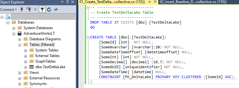
We’ll use our Azure SQL Database as the source again. So let’s create our TestDeltaLake source table, just like last time. As always, you can find the all the code in the GitHub repo.
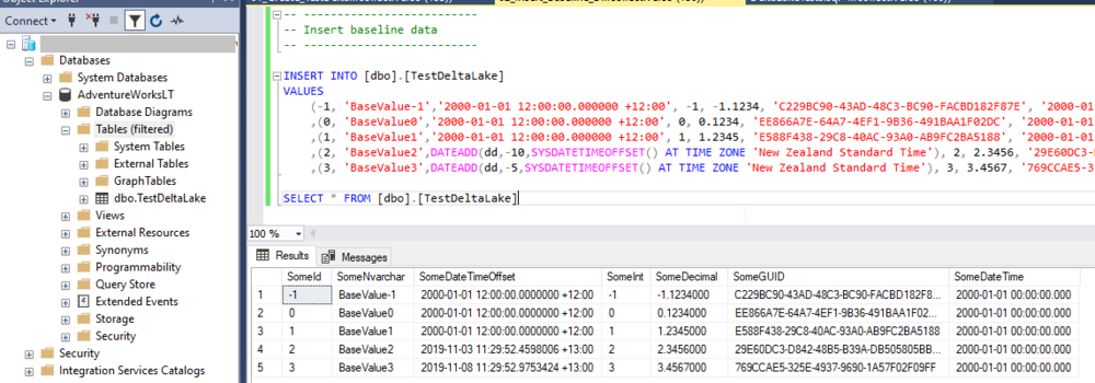
Add the baseline data.
To Databricks we go. If you’re using the same storage account and Databricks workspace as per the previous post, you’ll need to do some clean-up. Delete the folder that contains the data for Delta Table.

You’ll also need to delete the “table” in the Databricks workspace that was the reference to the data you just deleted in you storage account.

Now that the clean-up is done, we’ll move on to the notebook. The first area where you’ll notice some differences is in the variables section. We have a few more of them.
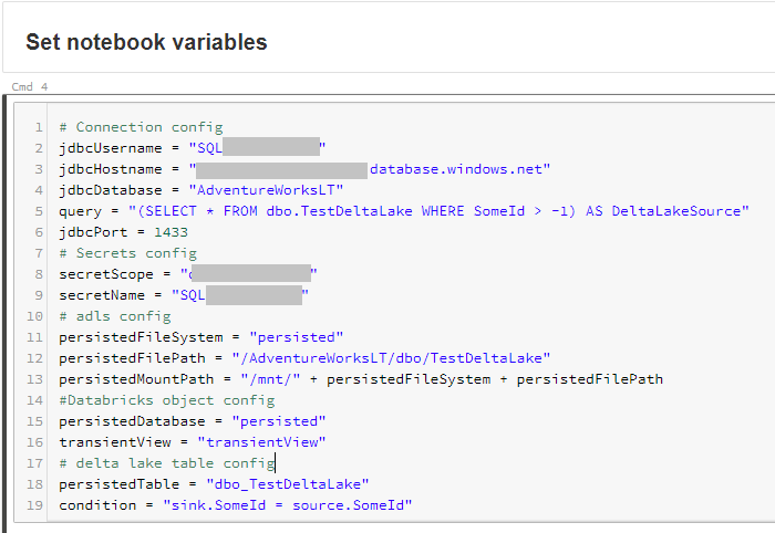
Specifically those required for ADLS, Databricks and the Delta Table config. These are:
persistedFileSystem: Name of the file system where we will store the data
persistedFilePath: The path within our file system where the data will live
persistedMountPath: As I mounted the file system, I can now use the “/mnt/” prefix so Databricks knows to write data to my external storage account. For more on mounting, see this post.
persisedDatabase: Name of the virtual database inside the Databricks workspace, I’ve kept it simple and went with “persisted” 🙂
transientView: Name of the view that will point to our source data. Again, I went with something generic, but call it what you want. I used “transientView” as this view commonly points to data stored in you transient data lake zone. In this case we’ve skipped that zone, but you get the point.
persistedTable: Name for the virtual table in the Databricks workspace
condition: The key on which the source to sink join will be performed. In the case of the TestDeltaLake table, the key is the SomeId column. This can happily be a composite key too, just stick to the sink.* = source.* structure and it works a treat.
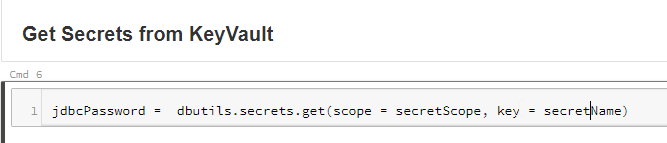
The next cell retrieves the password from the KeyVault secret and stores it in the jdbcPassword variable, exactly like last time.
Again we build the JDBC URL and set the connection properties.

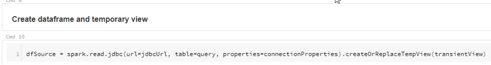
The next cell uses the JDBC connection and reads the data into a dataframe. It also creates a temporary view, aptly named “transientView” using our transientView variable.
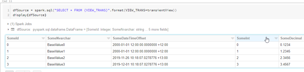
We can now query the temporary view just as before. We’re doing it a little differently this time by using string interpolation in pySpark (Python). Ultimately this builds and invokes the same SQL statement we had before, but it’s now dynamic SQL.
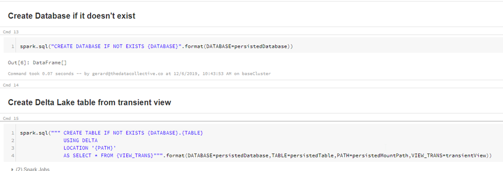
In the next set of cells, we create the “Persisted” Databricks database if it doesn’t exist, and then use a CTAS statement to create the dbo_TestDeltaLake Delta table in the persisted database. Again we use our string interpolation syntax.
As you can see when running the next cell, our Delta table contains the same data as our SQL table.

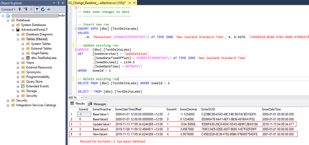
Let’s make the same changes as in the previous post.
In order to refresh our temporary view data, we need to run all the cells in the notebook up to and including “Show temporary view data”.

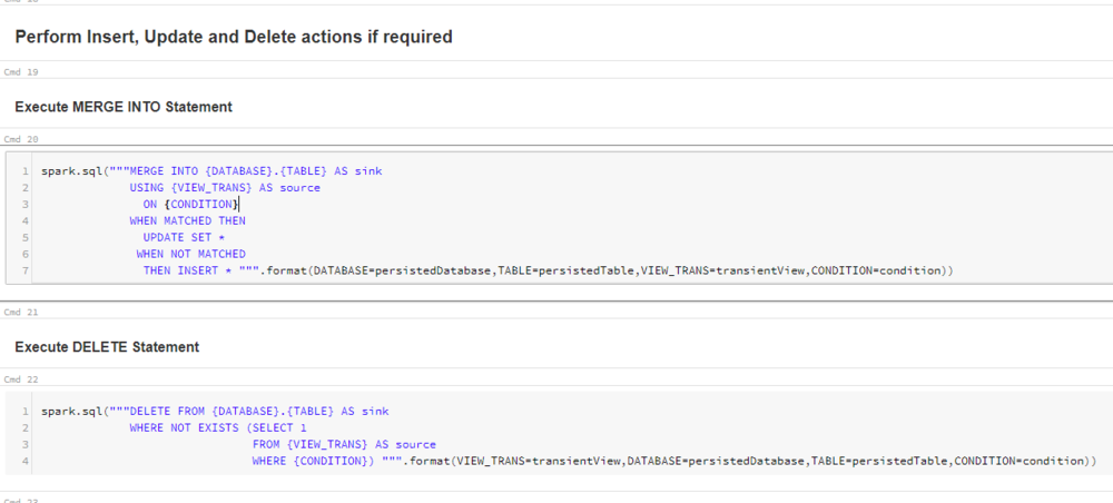
We can now run the next two cells which does a MERGE and DELETE respectively again using string interpolation.
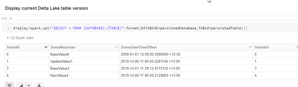
Just like last time, we can see that our Delta table now looks like our SQL source. The records where Merged and Deleted as we expected.
For the previous version, we once again see the records as it existed in the SQL Database when we initialised our table data.
Simple as that, you now have a dynamic notebook that will load any table from our Azure SQL Database source. We just need to set the variables in the first cell for the given table we want to load.
Now I know what you’re thinking, “but you hardcoded the variables”. Yes I did, deliberately! The last remaining thing to do is pass our notebook parameters rather than hardcode the variables. Notebook parameters are affectionately known as “widgets” in Databricks. I’m sure there’s a reason…
Widgets are beyond the scope of this post (only because they are super simple to set up), you can get all the details here. This example shows how I set up widgets in another notebook.

The beauty with this approach is that you can store the parameters you need in a metadata framework of whatever form, JSON, SQL, NoSQL, whatever. As look as you can look it up and pass it to your notebook, the notebook will take care of the rest.
Needless to say how you orchestrate this notebook is also up to you. Examples are Azure Data Factory, Logic Apps, Azure Functions or Databricks jobs with notebook chaining.
I hope you found the series helpful. Not sure what I’ll be writing about next, so I guess you’ll have to subscribe to the feed or keep an eye on twitter and LinkedIn for whatever’s next. Thanks for reading.
![]()