

Introduction
In Part I and Part II we covered some key MDX and cube concepts necessary for writing MDX even if you don’t have any cube development experience. We will cotinue the series by looking at some important MDX features and topics necessary for writing advanced MDX queries.
Please refer to Part I for the prerequisites needed to execute all MDX queries in this series.
Let’s say you get a request to generate a report like this:
Excluding California, find the top 10 all-time US states in reseller sales and for each of the ten states find the top 3 cities in reseller sales in the last two year and the percentage contribution of each of the city to their state's total?
Even though you could answer such requests with SQL queries, the response time will probably not be feasible if you are to parameterize the resulting query for an end-user report. This is especially true if the query has to ravage through millions, or even billions, of sales records. This is what Multidimensional modeling and MDX were designed for, and where MDX trump SQL.
Listing 1
WITH
SET qualifiedStates AS
  TopCount
    (
      Except
      (
        [Geography].[State-Province].Children
       ,[Geography].[State-Province].&[CA]&[US]

      )
     ,10
     ,[Measures].[Reseller Sales Amount]
    )

  SET TopCities AS
    Generate
   (
      CrossJoin
      (
        qualifiedStates
       ,tail([Date].[Calendar].[Calendar Year],2)
      )
     ,TopCount
      (
        CrossJoin
       (
         Descendants
          (
            [Date].[Calendar].CurrentMember
           ,[Date].[Calendar].[Calendar Year]
          )
         ,Descendants
          (
            [Geography].[Geography].CurrentMember
           ,[Geography].[Geography].city
          )
        )
       ,3
       ,[Measures].[Reseller Sales Amount]
      )
    )
  MEMBER [Measures].pctofState AS
      (
       [Geography].[Geography].CurrentMember
       ,[Measures].[Reseller Sales Amount]
      )
     /
      (
        [Geography].[Geography].CurrentMember.Parent
       ,[Measures].[Reseller Sales Amount]
      )
   ,format_string = '0.00%'
SELECT
  {
    [Measures].[Reseller Sales Amount]
   ,[measures]. pctofState
  } ON 0
 ,NON EMPTY
    CrossJoin
    (
      [Geography].[State-Province].Children
     ,{TopCities}
    ) ON 1
 FROM [Adventure Works]                                                  WHERE [Geography].[Country].&[United States];
Results:
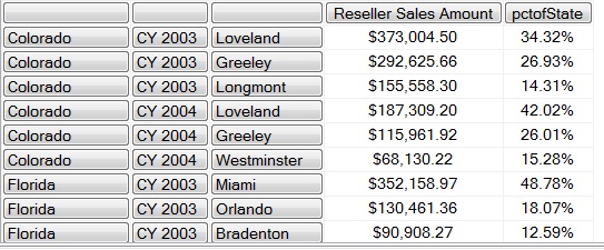
.........
The MDX query in Listing1 and the result above represent one solution to the sample request above. Now, let's proceed to look at the important MDX features that are necessary to accomplish such requests.
Calculated Members and Named Sets Using the “With” Keyword.
Just like SQL CTE’s, MDX uses the “WITH” Keyword to specify temporary calculations or sets defined within the execution scope of a SELECT Statement. In MDX you can define two types of expressions using the WITH keyword, namely Calculated Members and Named Sets.
A calculated member is an MDX member that is resolved by calculating an MDX expression to return a value.
A named set is resolved by returning a set expression, so unlike CTEs you must specify a “member” and “set” keywords in addition to the WITH clause for the Calculated Members and Named Set respectively.
The syntax of the WITH keyword is quite flexible just like in CTEs, for instance it allows a calculated member to be based on another calculated member or a named set. Let’s look at some examples.
Calculated Members
Listing 2 below shows a single calculated member called AverageResellerSales which resolves the ratio of sales amount to order count. The calculated member is then referenced in the select statement alongside other regular measures on the column axis.
Listing 2
with
member [AverageResellerSales] as
(
    [Measures].[Reseller Sales Amount]
   /[Measures].[Reseller Order Count]
)

 select
  {
     [Measures].[Reseller Sales Amount]
    ,[Measures].[Reseller Order Count]
    ,AverageResellerSales
  } on columns
 ,[Geography].[State-Province].members on rows
from  [Adventure Works]
Results:

Note that the member keyword was specified with the WITH keyword to indicate that it is a calculated Member. Let’s look at another example.
In listing 3 below, the AverageResellerSales calculated member from listing 2 above has been modified with an IIF statement to handle errors that may arise due to division-by-zero within calculated measures and the member name prefixed with “[Measures]” which is standard practice that says that the calculated member is of the measures hierarchy.
In the listing there is a second calculated member [Measures].[AverageResellerSales03] that calculates the same reseller ratio as the first member but only for the year 2003. The two calculated members are then referenced in the select statement alongside other regular measures on the columns axis. Some MDX formatting techniques has also been introduced here.
Listing 3
with
member [Measures].[AveResellerSales] as
IIF (
         [Measures].[Reseller Order Count]= 0
         , null
         ,(
          [Measures].[Reseller Sales Amount]
          /[Measures].[Reseller Order Count]
       )
) ,format_string = 'Currency'

member [Measures].[AveResellerSales03] as
(
  sum([Date].[Calendar Year].&[2003], [Measures].[Reseller Sales Amount])
  /sum([Date].[Calendar Year].&[2003] ,[Measures].[Reseller Order Count])
) ,  format_string = "$#,#.##"

 select
  {
    [Measures].[Reseller Sales Amount]
    ,[Measures].[Reseller Order Count]
    ,[Measures].[AveResellerSales]
   ,[Measures].[AveResellerSales03]
  } on columns
  ,[Geography].[State-Province].&[CA]&[US] on rows
 from  [Adventure Works]
Results:

Named Set
Listing 4 below shows an example of named set called TopSellingCities consisting of a set expression made up of three cities. The named set is then referenced in the select statement on the rows axis. Note that the set keyword is specified with the WITH keyword to indicate that it is a Named set.
Listing 4
with
set TopSellingCities
as {
       [Geography].[Geography].[City].&[Toronto]&[ON]
       ,[Geography].[Geography].[City].&[London]&[ENG]
       ,[Geography].[Geography].[City].&[seattle]&[WA]

   }

select
measures.[Reseller Sales Amount] on Columns
,TopSellingCities on rows
from [Adventure Works]
Results:

In the next example in listing 5 below, the TopSellingCities named set above is modified to a set that will always generate the top 3 cities in Sales (Reseller) by using the Topcount function. Note that just like calculated members, you can create more than one named set. The example below shows a named set in combination with a calculated member.
Listing 5
with
set TopSellingCities
as topcount(
             [Geography].[Geography].[City]
            ,3
            ,[Measures].[Reseller Sales Amount]
   )

member [Measures].[AveResellerSales] as
IIF (
         [Measures].[Reseller Order Count]=0
         , null
         ,(
          [Measures].[Reseller Sales Amount]
          /[Measures].[Reseller Order Count]
       )
) ,format_string = 'Currency'

select
{
   [Measures].[Reseller Sales Amount]
  ,[Measures].[AveResellerSales]
}on Columns
,TopSellingCities on rows
from [Adventure Works]
Results:

Iteration, Context awareness and the CurrentMember Function
In part II of this series, I explained the architecture of attribute and user-defined hierarchies and the implementation of member level in these hierarchies. In MDX the CurrentMember function is the function used to make calculations aware of the context of the query in which they are being applied. For instance, when iterating through a set of hierarchy members, at each step in the iteration, the CurrentMember function exposes the member being operated upon.
An example of how the CurrentMember function is used is seen in the example in listing 6 below. The first two calculated members show how to dynamically generate parent and child Reseller sales amounts for any member of the geography hierarchy. Note also that because the two calculated members are used to resolve the third calculated member, the ratio will also be in the context of the current member. The context of the result of the query in this case will be driven by the members of the geography hierarchy displayed on the rows axis.
Listing 6
with
member [Measures].[ChildSalesAmount]
as sum(

        [Geography].[Geography].CurrentMember
        ,measures.[Reseller Sales Amount]
   )


 member [Measures].[ParentSalesAmount]
  as sum(
    [Geography].[Geography].CurrentMember.Parent
   , [Measures].[Reseller Sales Amount]
   )


member [Measures].[ChildParentRatio]
  as    [Measures].[ChildSalesAmount]
        /[ParentSalesAmount], format_string = '0.000'


select
 {
    ParentSalesAmount
    ,ChildSalesAmount
    ,ChildParentRatio
 } on columns,

[Geography].[State-Province].Children  on rows
--[Geography].[City].children on rows
FROM [Adventure Works]
Result:
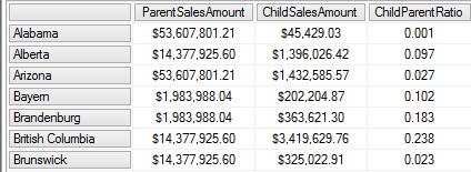
………
Because the members from the state-province are displayed on the rows axis, the ChildSalesAmount consist of the state-province sales amounts and the ParentSalesAmount consist of the country sales amounts. Watch how the context and resulting calculation changes If you comment out the state-province members and uncomment the city members on the rows axis.
Aggregation and Statistical functions
I introduced the sum aggregation function in listing 3 above. Most of the MDX aggregation functions have a similar operation. They return a numeric expression of the aggregation type (Sum, Max, Avg etc.) over a specified set. The general syntax is as below.
Aggregation_Function_Name( Set_Expression [ , Numeric_Expression ] )
The specific functions may have slight syntax variations. Remember to refer to the MDX function List for exact variations of the use of these functions.
In the example in listing 7 below, a named set Duration consisting of 24 months is created and referenced in each of the calculated members. In the calculated members the numeric expression [Measures].[Reseller Sales Amount] is evaluated across the set and then the aggregation function is applied.
Listing 7
WITH Set Duration as
([Date].[Calendar].[Month].&[2001]&[7] : [Date].[Calendar].[Month].&[2003]&[6])
MEMBER [measures]._Total
AS sum
 (
Duration
       ,[Measures].[Reseller Sales Amount]
)

MEMBER [measures]._Avg
 AS
 Avg (
        Duration
        ,[Measures].[Reseller Sales Amount]
      )
MEMBER [measures]._Cnt
 AS
 count (
        Duration
      )

 SELECT {

 [measures]._Total
,[measures]._Cnt
,[measures]._Avg

} ON 0

FROM [Adventure Works]
Result:
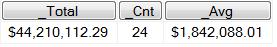
Note that if a numeric expression is not specified in the aggregation function, then the result is evaluated in the context of the members of the sets on the query axis before the aggregation is applied. For instance the example in listing 8 below generates a hierarchal statistical summary. Because numeric expression are not specified in each of the aggregation function, they are evaluated in the context of the currentmember of date hierarchy on the rows axis and the order count numeric expression passed in the where clause.
Listing 8
WITH MEMBER [Date].[Date]._Total
AS sum
( descendants(
               [Date].[Calendar].CurrentMember
               ,[Date].[Calendar].[Date]
               )
)

MEMBER [Date].[Date]._Cnt
 AS
Count ( descendants(

               [Date].[Calendar].CurrentMember
               ,[Date].[Calendar].[Date]
               )
)

MEMBER [Date].[Date]._Max AS
Max
 ( descendants(

               [Date].[Calendar].CurrentMember
               ,[Date].[Calendar].[Date]
               )
   )

MEMBER [Date].[Date]._Min AS
Min( descendants(

               [Date].[Calendar].CurrentMember
               ,[Date].[Calendar].[Date]
               )
   )

MEMBER [Date].[Date]._Med AS
Median ( descendants(

               [Date].[Calendar].CurrentMember
               ,[Date].[Calendar].[Date]
               )
   )

MEMBER [Date].[Date]._Avg
AS
Avg (  descendants(
               [Date].[Calendar].CurrentMember
               ,[Date].[Calendar].[Date]
               )
   )
MEMBER [Date].[Date]._Stdev AS
Stdev  (
         descendants(
               [Date].[Calendar].CurrentMember
               ,[Date].[Calendar].[Date]
               )

   ), format_string='#'

SELECT {

  [Date].[Date]._min
, [Date].[Date]._max
, [Date].[Date]._Total
, [Date].[Date]._Cnt
, [Date].[Date]._Avg
, [Date].[Date]._Med
, [Date].[Date]._Stdev

} ON columns

,NON EMPTY [Date].[Calendar].[Calendar Year].members
ON rows
FROM [Adventure Works]
where ([Measures].[Order Count])
Results:

Set Functions
Topcount
The Topcount() function introduced in listing 5 above implicitly sorts a set in descending order and returns a specified number of elements passed as argument from the top. The three arguments passed in are a set expression, the number of elements to be returned, and the numeric expression of the members to be returned.
TopCount(Set_Expression, count, Numeric_Expression)
For instance the example in listing 9 returns the top 3 all-time countries in resellers sales.
Listing 9
SELECT [Measures].[Reseller Sales Amount] ON 0,
TopCount
   ([Geography].[Geography].[Country].Members
   , 3
   , [Measures].[Reseller Sales Amount]
  ) ON 1

FROM [Adventure Works]
Results:

Note that any legitimate set and numeric expressions can be passed to the function. For instance listing 10 below returns the top 3 countries in resellers sales plus taxes for the last calendar year. Note the use of the Tail() function to return the last calendar year.
Listing 10
SELECT [Measures].[Reseller Sales Amount] ON 0,
TopCount
   (crossjoin
              (
                 [Geography].[Geography].[Country].Members
                 ,tail([Date].[Calendar].[Calendar Year],1 )
               )
   , 3
   , ([Measures].[Reseller Sales Amount]+[Measures].[Reseller Tax Amount])
   ) ON 1
FROM [Adventure Works]
Results:

TopPercent
The TopPercent function implicitly sorts a set in descending order and calculates the sum of the specified numeric expression evaluated over the specified set. The function then returns the elements with the highest values whose cumulative percentage of the total summed value is at least the specified percentage. The resulting elements are returned ordered from the largest to smallest.
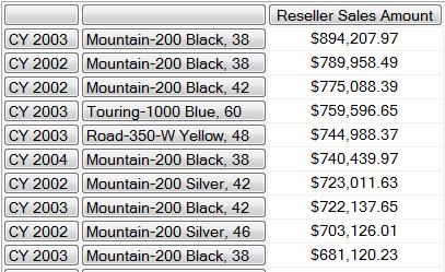
In the example in listing 11, the products which constitute twenty percent of Reseller sales in each year are generated using the TopPercent function.
Listing 11
SELECT
  [Measures].[Reseller Sales Amount] ON 0
 ,Generate
  (
    [Date].[Calendar].[Calendar Year].MEMBERS
   ,TopPercent
    (
      crossjoin(
        [Date].[Calendar].[Calendar Year].MEMBERS
        ,[Product].[Product Categories].[Product]
      )
     ,20
     ,[Measures].[Reseller Sales Amount]
    )
  ) ON 1
FROM [Adventure Works];
Results:
Similar in operation to the TopCount and TopPercent functions are the TopSum, BottomCount, BottomSum and the BottomPercent functions. For these and a complete list and usage of all MDX functions please refer to this http://msdn.microsoft.com/en-us/library/ms144792.aspx.
Assigning Ranks
Another inescapable aspect of advanced data analysis is ranking of data. Ranking functions present results in a specified order with or without the ordinal or rank numbers assigned to the row in the resultset. The TopCount function introduced above is an example of the latter. To assign rank numbers to an ordered set you have to use the Rank function. Note that the Rank function just assigns the ordinal numbers so the set supplied to the Rank function must be ordered. On MSDN the syntax for the rank function is shown below.
Rank(Tuple_Expression, Set_Expression [ ,Numeric_Expression ] )
From the syntax we can rank resellers based on their 2003 sales as in listing 12 below.
Listing 12
WITH
  MEMBER [Measures].[ResellerRnk] AS
    Rank
    (
     [Reseller].[Reseller].CurrentMember
     ,Order
      (
       [Reseller].[Reseller].[Reseller].MEMBERS
       ,[Measures].[Reseller Sales Amount]
       ,BDESC
      )
    )
SELECT
  [Measures].[ResellerRnk] ON 0
,[Reseller].[Reseller].[Reseller].MEMBERS ON 1
FROM [Adventure Works]
WHERE [Date].[Calendar].[Calendar Year].&[2003];
Results:

………
The query runs and returns the rank, but there is a severe performance penalty with this implementation. Because the reseller members are evaluated in the current context, the ordering of employees is done for every single cell where the calculated member is evaluated.
You can read more about this performance issue and a lot of other MDX techniques at Mosha’s blog at http://sqlblog.com/blogs/mosha/archive/2006/03/14/ranking-in-mdx.aspx
To side step the ranking performance issues inherent in the query in listing 12, first we have to order the set outside the rank function before you passing it to the rank function as shown in listing 13 below. This way the set is only ordered only once.
Listing 13
WITH
  SET OrdResellers AS
    Order
    (
      [Reseller].[Reseller].[Reseller].MEMBERS
     ,[Measures].[Reseller Sales Amount]
     ,BDESC
    )

  MEMBER [Measures].[ResellerRnk] AS
    Rank
    (
      [Reseller].[Reseller].CurrentMember
     ,OrdResellers
    )

SELECT
  [Measures].[ResellerRnk] ON 0
 ,[Reseller].[Reseller].[Reseller].MEMBERS ON 1
FROM [Adventure Works]
WHERE [Date].[Calendar].[Calendar Year].&[2003];
Results:

......
To highlight the performance gain between the two queries, the query in listing 12 took 19 sec 276 ms to run on my old laptop, but the query in listing 13 took a mere 88 ms to run. Remember to always order a set before you pass it to the rank function.
Filtering data
We encountered the MDX WHERE and HAVING clause in Part 1 and noted how both clauses works almost like their SQL counterparts. I also introduced the IIF function in listing 3 where it was used to handle errors that may arise due to division-by-zero within a calculated member.
The Filter function
The Filter function is similar in logical operation to the IIF function but takes only two arguments and returns a set that meet the specified search condition. It automatically returns null where the search conditions are not met. The syntax for the filter function is a below.
Filter(Set, LogicalExpression )
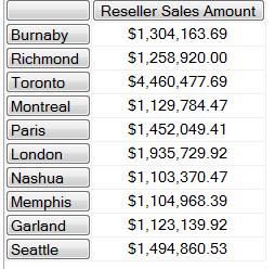
In the example in listing 14 below the filter function is used on the rows axis to return cities with a million or more in reseller sales.
Listing 14
SELECT
  [Measures].[Reseller Sales Amount] ON 0
 , NON EMPTY
Filter
  (
    [Geography].[Geography].[City].MEMBERS
   ,[Measures].[Reseller Sales Amount] >= 1000000
  ) ON 1
FROM [Adventure Works];
Results:
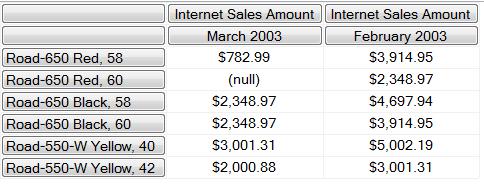
The set can be any well formulated set, and the logical expressions may also include aggregations and MDX operands as shown in the example in listing 15 below. The query displays products with fewer sales in February 2003 than in January 2003 and also sold less than $5000.
Listing 15
with set FilteredSet as
NON EMPTY
Filter
  (
    [Product].[Product].Children
   , (  Sum
        (
         [Date].[Calendar].[Month].&[2003]&[3]
        ,[Measures].[Internet Sales Amount]

        )
     <
        Sum
        (
          ParallelPeriod ([Date].[Calendar].[Month]
          , 1
           , [Date].[Calendar].[Month].&[2003]&[3])
         ,[Measures].[Internet Sales Amount]
        )
    AND
        Sum
        (
         [Date].[Calendar].[Month].&[2003]&[3]
         ,[Measures].[Internet Sales Amount]
        )
      < 5000
     )
)

SELECT
    ({[Measures].[Internet Sales Amount]}
    *
    {
      [Date].[Calendar].[Month].&[2003]&[3], [Date].[Calendar].[Month].&[2003]&[2]
    } )ON COLUMNS
, FilteredSet ON ROWS
FROM [Adventure Works];
Results:
The Case Statement
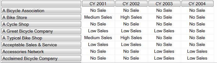
The Case statement in MDX works the same as in SQL. Case statements are useful in filtering data into segments or for converting continuous or discrete values to categorical data. Examples are shown in listing 16 and listing 17 below.
Listing 16
WITH MEMBER [Measures].AnnualResellerSales As
CASE
   WHEN [Measures].[Reseller Sales Amount] > 750000 THEN 'Very High Sales'
   WHEN [Measures].[Reseller Sales Amount] > 50000 THEN 'High Sales'
   WHEN [Measures].[Reseller Sales Amount] > 25000 THEN 'Medium Sales'
   WHEN [Measures].[Reseller Sales Amount] > 0 THEN 'Low Sales'

   ELSE 'No Sale'
 END
SELECT  [Date].[Calendar].[Calendar Year].members on 0
,NON EMPTY [Reseller].[Reseller].children on 1
FROM [Adventure Works]
WHERE [Measures].AnnualResellerSales
Results:
Listing 17
WITH MEMBER [Measures].[ResellerOrderCnt] AS
CASE [Measures].[Reseller Order Count]
   WHEN 0 THEN 'None'
   WHEN 1 THEN 'Very Low'
   WHEN 2 THEN 'Low'
   WHEN 3 THEN 'Low'
   WHEN 4 THEN 'Intermediate'
   WHEN 5 THEN 'High'
   WHEN 6 THEN 'High'
      ELSE 'Very High'
END

SELECT [Geography].[Geography].[State-Province].Members on rows
,NON EMPTY
 Calendar.[Calendar Year] on columns
FROM [Adventure Works]
WHERE [Measures].[ResellerOrderCnt]
Results:

Running MDX queries using SQL Store Procedures
You may encounter some complex reporting needs where parameterizing MDX is not enough or third party applications inhibit using MDX directly. In some of these cases retrieving the tabular cube data through SQL Server stored procedures could be very handy. This option also allow you write complex dynamic MDX queries where necessary. Note there may some bottlenecks and performance hits using linked servers, which is a requirement for this method, so consider this approach if it is best solution available.
Because the stored procedure will be running in SQL Server, we first need to set up a link server. Once the linked server is setup we can use the OpenQuery method as below.
Select *
 From OpenQuery('SSASLinkedServerName', 'mdxQuery')
Linked servers can be setup manually through SSMS as shown in this link http://www.sqlservercentral.com/articles/Distributed+Queries/linkedserver/139/ or with a script as shown in listing 18 below. In the example a new linked server called SSAS_Linked_Srv_Local is setup on a local server if it doesn’t already exist. The script proceeds to create a stored procedure up.SSAS_GET_ResellerSales which takes two parameters: a reseller name and a year. The parameters are passed dynamically within the MDX query that gets executed to generate monthly sales for the particular reseller in the year that was passed to the store procedure.
Listing 18
IF NOT EXISTS (SELECT s.name
FROM sys.servers s
WHERE s.server_id != 0
AND s.name = 'SSAS_Linked_Srv_Local'
)
EXEC sp_addlinkedserver
@server= 'SSAS_Linked_Srv_Local',
@srvproduct='',
@provider='MSOLAP',
@datasrc='(Local)',
@catalog='AdventureWorksDW'
CREATE PROCEDURE up.SSAS_GET_ResellerSales
@reseller nvarchar(200)
,@year nchar(4)
AS
BEGIN
declare
@linkedServer as varchar(max)
,@mdx as varchar(max)
,@query as nvarchar(max)
set @mdx = 'with member [Measures].[ResellerSales]
as
IIF ( [Measures].[Reseller Sales Amount] > 0
,[Measures].[Reseller Sales Amount]
,0)
select
[Measures].[ResellerSales] on 0
,[Date].[Calendar].[Month] on 1
from [Adventure Works]
where ([Reseller].[Reseller].['+ @reseller +']
,[Date].[Calendar Year].&['+ @year + ']);'
set @linkedServer = 'SSAS_Linked_Srv_Local'
set @query = 'SELECT * FROM OpenQuery('+@linkedServer+','''+ @mdx +''')'
execute sp_executesql @query
END
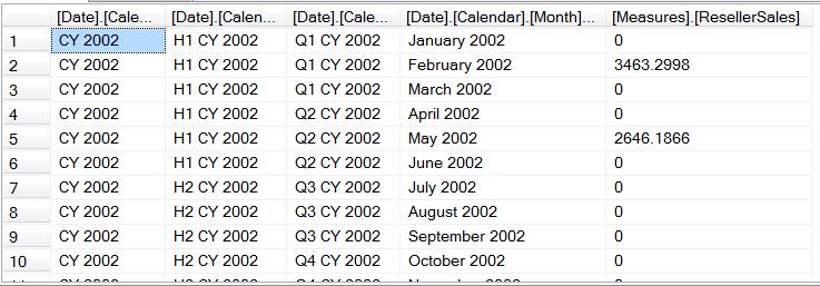
GOA sample execution of the stored procedure created above is shown below. Remember to execute the query in listing 18 and listing 19 as SQL queries and not as MDX queries.
Listing 19
exec up.SSAS_GET_ResellerSales 'Alternative vehicles', '2002'
Results:
Conclusion
This brings us to the conclusion of this series. In this final part we explored important MDX features necessary for advanced MDX analysis, note however that many other topics and MDX functions were not covered in these series. Please refer to appropriate resources for other advanced topics. Also refer to the MDX function list http://msdn.microsoft.com/en-us/library/ms144792.aspx for syntax and used of functions not covered.