

Attached as a resource to this article is an MS DOS application I wrote a few years ago in Microsoft QuickBASIC and assembly language that displays a functioning artificial neural network (ANN) and illustrates the underlying mathematics.
While the operating system and code are obsolete, the math is not.
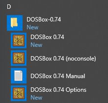
Executing the DOS Optical Character Recognition (OCR) Demo Application
- Download and install the free DOSBox DOS-emulator from http://dosbox.com.
- Create a folder C:\OCR
- Download and extract the attached OCR.zip resource file to the C:\OCR folder.
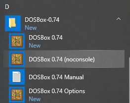
- Start the "noconsole" version of DOSBox.
- Mount the C:\OCR folder as drive c.
- Switch to the mounted C drive.
- Execute the ocr.exe application.
2. The Optical Character Recognition Artificial Neural Network in Action
- A splash screen comes up for a few seconds.

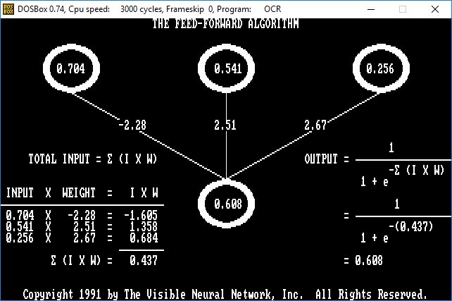
- The next screen shows the mathematics of the feed-forward algorithm.
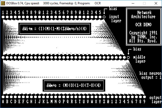
- The following screen shows the architecture of the OCR ANN, and the mathematics of the error back-propagation algorithm for incremental correction of the input and output layers of connection weights.
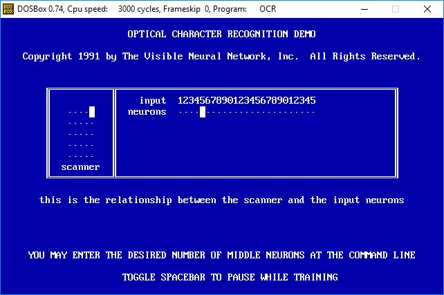
- The alphanumeric character scanner and its relation to the input neurons is shown next.
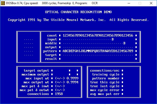
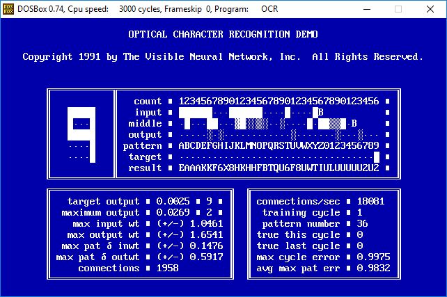
- This screen shows the network monitoring panel before the first pattern is scanned. At this point all the connection weights have been randomly set to the range -1.0000 to +1.0000 as seen in the max input wt and max output wt fields.
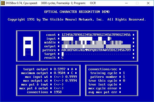
- The first pattern, the alphanumeric character "A," is scanned. The input neurons are given the value 1 for pixels that are activated by the character and 0 for the pixels that are not. In a perfectly trained neural network the "A" output neuron would have an activation value of one and all the other output neurons would have an activation value of zero. The middle and output neuron values are calculated via the feed-forward algorithm from the scanned values in the input neurons. On this first pattern of the training cycle almost all of the output neurons compute to some non-zero value. Even though the letter "A" was scanned, the output neuron with the highest activation value is the one represented by "C" as shown by the target output and maximum output fields. Each time a pattern is entered the connection weights will be adjusted in proportion to the amount that each connection is contributing to the error via the back-propagation algorithm. The error for each output neuron is the amount that it differs from its target value.
- After scanning through all 36 input patterns the network has not correctly identified a single character. The maximum error this cycle was 0.9975, and the average error was 0.9832 as shown in the max cycle error and avg max pat err fields. Note also that the maximum input weight change on a character pattern was 0.1476 and the maximum output weight change was 0.5917 for the first training cycle.
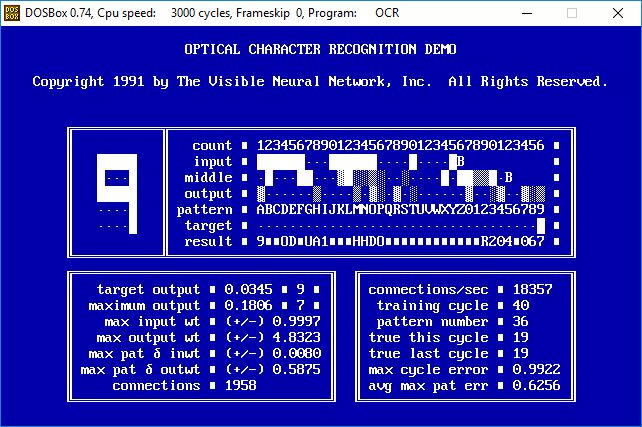
- After 40 training cycles the neural network is identifying 19 of 36 characters correctly, and the average pattern error has decreased by a third.
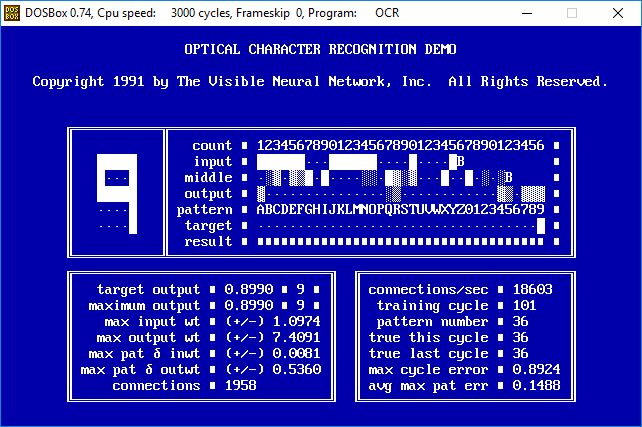
- After 101 training cycles the network identifies all 36 characters correctly, and the average pattern error is down to 0.1488.
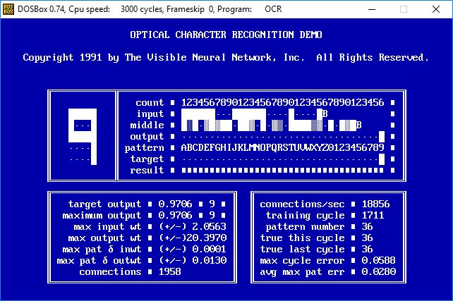
- After hundreds of training cycles the average pattern error has decreased to 0.0280 and the activation values of the target neurons when each pattern is scanned is approaching 1.0000. Note also that the maximum absolute input weight has increased to 2.0563 and the maximum absolute output weight has increased to 20.3970.
The Mathematics of an Artificial Neural Network
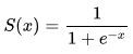
A neuron accepts one or more input signals through connections to other neurons or outside stimuli, sums them up and transforms them into an output signal. The sum of the input signals can range from negative to positive infinity. The output (activation) signal can range from zero to one. The most common mathematical transform function used to emulate a biological neuron activation signal is the sigmoid function:
 (from Wikipedia)
When using the sigmoid function to calculate the activation signal of a neuron, the variable x is replaced with the sum of the input signals.
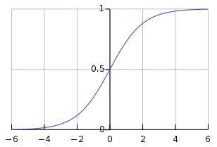
This graph of the sigmoid function displays the sum of the input signals on the x-axis and the resulting output activation signal on the y-axis.
 (from Wikipedia)
When the sum of the input signals is below 6, the output is essentially 0. When the sum of the input signals is 0, the output signal is 0.5. When the sum of the input signals is above 6, the output is essentially 1. In the range of summed input signals between negative and positive 6 the output increases logarithmically from zero to one with an inflection point at y = 0.5.
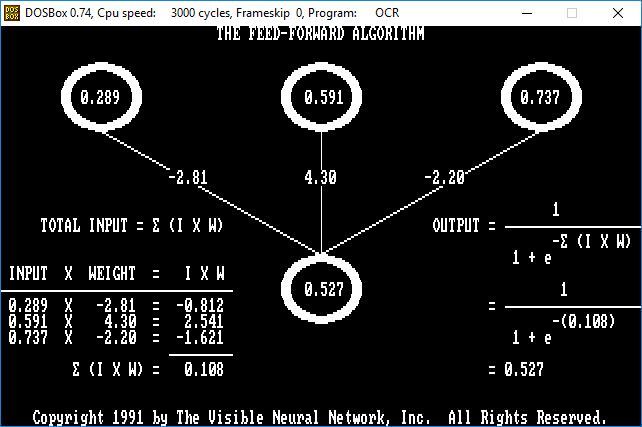
The Feed-Forward Algorithm: Calculating a Neuron Activation Value
In the illustration below, three input neurons of varying activation magnitudes I are connected to an output neuron via connections of varying weighting factors W to yield an activation signal in the output neuron that is computed using the sigmoid function.
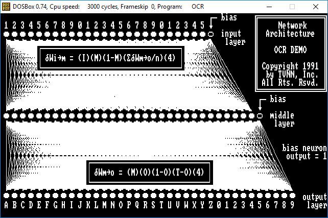
Artificial Neural Network Architecture
The most common artificial neural network design consists of three layers of neurons: an input layer, a middle layer and an output layer. The first two layers also contain a bias neuron, a neuron which has a constant activation value of one. Each neuron in an upper layer is connected to each neuron in the succeeding layer. The number of neurons to configure in the middle layer is commonly determined by adding the number of neurons in the input layer and output layer and dividing by two.
Before training begins, each of the connection weights is randomly set within the range minus one to plus one.
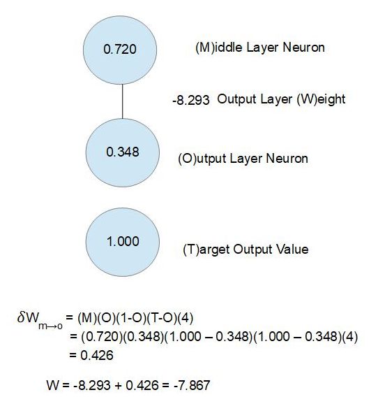
Back-Propagation Calculation of the Correction Factor for an Output Layer Connection
The back-propagation equation...
δWm→o = (M)(O)(1-O)(T-O)(4)
...calculates the amount that a connection weight between a middle neuron and an output neuron should be changed based on the difference between the output neuron's activation value and its target value when each character is scanned.
In the illustration below, the correction factor is calculated as 0.426 and the connection weight will be changed from -8.293 to -7.867.
Back-Propagation Calculation of the Correction Factor for an Input Layer Connection
The back-propagation equation for the input layer of weights differs from that of the output layer weights...
δWi→m = (I)(M)(1-M)(ΣδWm→o/n)(4)
...where the error calculation (T-O) is replaced with (ΣδWm→o/n), which is the average weight change of the output layer connections to the middle neuron.
In the illustration below, an input neuron is connected to a middle neuron that is in turn connected to three output neurons.
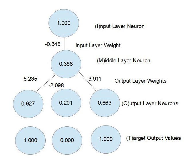
The correction factors for the three output connections are calculated as before:
(M)(O)(1-O)(T-O)(4) =
(0.386)((0.927)(1 - 0.927)(1 - 0.927)(4) = 0.008
(0.386)(0.201)(1 - 0.201)(0.-0.201)(4) = -0.050
(0.386)(0.663)(1 - 0.663)(1 - 0.663)(4) = 0.116
---------
0.074
Add them together and divide by 3 to arrive at the average correction factor = 0.074 / 3 = 0.025.
Compute the input layer weight correction factor as:
δWi→m = (I)(M)(1-M)(ΣδWm→o/n)(4) =
(1.000)(0.386)(1 - 0.386)(0.025)(4) = 0.237
The input layer weight will be changed to (-0.345 + 0.237) = -0.108.
Conclusion
The purpose of this article has been to show an artificial neural network in action and illuminate the underlying mathematics rather than dwell on theory.
In purely mathematical terms an artificial neural network is a set of simultaneous non-linear equations with an infinite set of acceptable solutions.
Training an artificial neural network is incremental iteration toward an increasingly better solution set for the set of simultaneous non-linear equations.
In practice it is not necessary to perform back-propagation on the input layer of weights. The input layer of connection weights is primarily a mixer. Back-propagation on the output layer of weights alone will usually result in a trained network.