

I know I have been light on blog posting this year. They always say that life tends to get in the way of these sorts of tasks, and this year that is certainly true. Anyways, I want this blog to be more than just SQL Server virtualization with VMware vSphere, so I’m intending to branch out – not just with more hypervisors (Microsoft Hyper-V 2012 tips and tricks coming soon!) but want some more fun tidbits about core SQL Server as well.
So… a few days ago one of my favorite clients passed on a question from one of his other consultants. The question was – “Why is ‘greater than’ and ‘less than’ faster than ‘ between’ for range filters in where clauses?”
What a great question! Let’s experiment and see what conclusions we can draw.
I’ll test with date ranges.
First, let’s create a container to test with. Pick any throw-away database and let’s get started!
- --create container for our dummy data
- CREATE TABLE [dbo].[BTW](
- [ID] [int] IDENTITY(1,1) NOT NULL,
- [DT] [datetime] NULL,
- CONSTRAINT [PK_BTW] PRIMARY KEY CLUSTERED
- (
- [ID] ASC
- )WITH (PAD_INDEX = OFF, STATISTICS_NORECOMPUTE = OFF, IGNORE_DUP_KEY = OFF, ALLOW_ROW_LOCKS = ON, ALLOW_PAGE_LOCKS = ON, FILLFACTOR = 100) ON [PRIMARY]
- ) ON [PRIMARY]
Now, we’ll prime the table with some random date values. This script was adapted from a script from Ben Nadel.
- --prime table with random date values.
- --script adapted from http://www.bennadel.com/blog/310-Ask-Ben-Getting-A-Random-Date-From-A-Date-Range-In-SQL.htm
- declare @i int
- set @i = 1
- -- First, let's declare the date range. I am declaring this
- -- here for the demo, but this could be done anyway you like.
- DECLARE @date_from DATETIME;
- DECLARE @date_to DATETIME;
- -- Set the start and date dates. In this case, we are using
- -- the month of october, 2006.
- SET @date_from = '1900-01-01';
- SET @date_to = '1999-12-31';
- while (@i < 100000) begin
- -- Select random dates.
- insert into dbo.btw (DT)
- SELECT
- (
- -- Remember, we want to add a random number to the
- -- start date. In SQL we can add days (as integers)
- -- to a date to increase the actually date/time
- -- object value.
- @date_from +
- (
- -- This will force our random number to be GTE 0.
- ABS(
- -- This will give us a HUGE random number that
- -- might be negative or positive.
- CAST(
- CAST( NewID() AS BINARY(8) )
- AS INT
- )
- )
- -- Our random number might be HUGE. We can't have
- -- exceed the date range that we are given.
- -- Therefore, we have to take the modulus of the
- -- date range difference. This will give us between
- -- zero and one less than the date range.
- %
- -- To get the number of days in the date range, we
- -- can simply substrate the start date from the
- -- end date. At this point though, we have to cast
- -- to INT as SQL will not make any automatic
- -- conversions for us.
- CAST(
- (@date_to - @date_from)
- AS INT
- )
- )
- )
- set @i = @i + 1
- end
OK. Run the block a few times to get a good number of rows in your test table. For the numbers below, I am running these on my home lab with SQL Server 2008R2 and 736,000 records in this table. I’ll just pluck some random dates out of thin air and off we go.
- set statistics io on
- set statistics time on
- select * from dbo.BTW where DT between '1945-01-08' and '1965-01-01'
- select * from dbo.BTW where DT >= '1945-01-08' and DT <= '1965-01-01'
- set statistics io off
- set statistics time off
We see some interesting results.
- (147622 row(s) affected)
- Table 'BTW'. Scan count 1, logical reads 1252, physical reads 0, read-ahead reads 0, lob logical reads 0, lob physical reads 0, lob read-ahead reads 0.
- SQL Server Execution Times:
- CPU time = 47 ms, elapsed time = 1483 ms.
- SQL Server parse and compile time:
- CPU time = 0 ms, elapsed time = 0 ms.
- (147622 row(s) affected)
- Table 'BTW'. Scan count 1, logical reads 1252, physical reads 0, read-ahead reads 0, lob logical reads 0, lob physical reads 0, lob read-ahead reads 0.
- SQL Server Execution Times:
- CPU time = 47 ms, elapsed time = 1964 ms.
- SQL Server parse and compile time:
- CPU time = 0 ms, elapsed time = 0 ms.
I have identical output here for each query. I ran this twenty times and got relatively the same results each time. The query execution plans are identical as well.
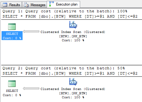
Hover over the Clustered Index Scan for each query. They are identical. It even converted the between to GTE and LTE for you. Sweet.
These look identical. So… why are the runtimes consistently different? What if we change the order of the queries? What about cleaning up memory to make sure we have no background ‘stuff’ getting in the way? (Don’t run those commands on production!)
- --test queries
- DBCC FREEPROCCACHE
- DBCC DROPCLEANBUFFERS
- set statistics io on
- set statistics time on
- select * from dbo.BTW where DT >= '1945-01-08' and DT <= '1965-01-01'
- select * from dbo.BTW where DT between '1945-01-08' and '1965-01-01'
- set statistics io off
- set statistics time off
Even more strange. The runtimes stayed with the locations and not the queries. It just gives us some proof that these really are equivalent.
Maybe we should create an index on the column we’re filtering on? Let’s try it.
- --add a nonclustered index on DT column.
- create nonclustered index IX_BTW_DT on dbo.BTW (DT) with ( fillfactor = 50 )
- --lots of room for inserts, as this is random data.
- --rerun queries.
- set statistics io on
- set statistics time on
- select * from dbo.BTW where DT between '1945-01-08' and '1965-01-01'
- select * from dbo.BTW where DT >= '1945-01-08' and DT <= '1965-01-01'
- set statistics io off
- set statistics time off
Did it make a difference in the queries? Nope. The only thing that changed was the number of logical reads. Run them in reverse or forward order and these came out all over the place.
- SQL Server parse and compile time:
- CPU time = 0 ms, elapsed time = 0 ms.
- (147622 row(s) affected)
- Table 'BTW'. Scan count 1, logical reads 663, physical reads 0, read-ahead reads 0, lob logical reads 0, lob physical reads 0, lob read-ahead reads 0.
- SQL Server Execution Times:
- CPU time = 32 ms, elapsed time = 800 ms.
- SQL Server parse and compile time:
- CPU time = 0 ms, elapsed time = 0 ms.
- (147622 row(s) affected)
- Table 'BTW'. Scan count 1, logical reads 663, physical reads 0, read-ahead reads 0, lob logical reads 0, lob physical reads 0, lob read-ahead reads 0.
- SQL Server Execution Times:
- CPU time = 47 ms, elapsed time = 1922 ms.
- SQL Server Execution Times:
- CPU time = 0 ms, elapsed time = 0 ms.
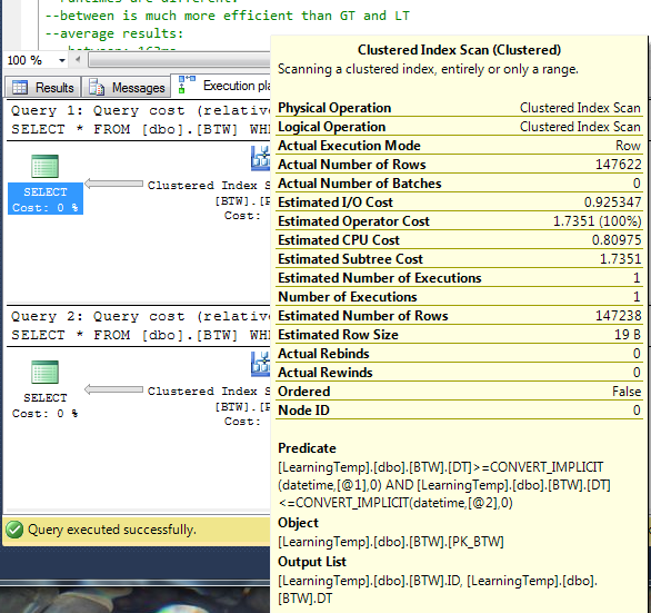
Now, notice something with the above screenshot of the execution plan. We’ve got implicit conversions on the date! Ack! If you ever see those in your query execution plans, figure out what’s going on and fix it. It’s extra overhead and might not always work the way you expect. Jes Borland has a great writeup on how to detect and correct implicit type conversions. It’s a great read!
I also tinkered around by putting a delay in between the two queries in an attempt to separate them a bit more.
- --implicit type conversions in the queries above? fix them!
- set statistics io on
- set statistics time on
- select * from dbo.BTW where DT between cast('1945-01-08' as datetime) and cast('1965-01-01' as datetime)
- waitfor delay '00:00:05'
- select * from dbo.BTW where DT >= cast('1945-01-08' as datetime) and DT <= cast('1965-01-01' as datetime)
- set statistics io off
- set statistics time off
That fixed the differences in runtimes. Now these are spaced out and the queries are executing almost identically.
- SQL Server parse and compile time:
- CPU time = 0 ms, elapsed time = 0 ms.
- (147622 row(s) affected)
- Table 'BTW'. Scan count 1, logical reads 663, physical reads 0, read-ahead reads 0, lob logical reads 0, lob physical reads 0, lob read-ahead reads 0.
- SQL Server Execution Times:
- CPU time = 47 ms, elapsed time = 1280 ms.
- SQL Server Execution Times:
- CPU time = 0 ms, elapsed time = 5001 ms.
- SQL Server parse and compile time:
- CPU time = 0 ms, elapsed time = 0 ms.
- (147622 row(s) affected)
- Table 'BTW'. Scan count 1, logical reads 663, physical reads 0, read-ahead reads 0, lob logical reads 0, lob physical reads 0, lob read-ahead reads 0.
- SQL Server Execution Times:
- CPU time = 16 ms, elapsed time = 1127 ms.
- SQL Server Execution Times:
- CPU time = 0 ms, elapsed time = 0 ms.
Now, are these results conclusive to where I can objectively state that one is faster than the other? Of course not. Between is just shorthand for GTE and LTE anyways. Between looks to be translated to GTE and LTE during query compilation, and the execution plan reflects GTE and LTE. The execution times should be the same, give or take background noise on the server.
One thing to keep in mind with BETWEEN is how you might get some skewed filtered data if you are not careful. Between is technically greater than and equal to PLUS less than and equal to. If you are using date ranges like the examples above, your filter translates to:
- select * from dbo.BTW where DT between cast('1945-01-08' as datetime) and cast('1965-01-01' as datetime)
- --translates to:
- select * from dbo.BTW where DT >= cast('1945-01-08 00:00:00' as datetime) and DT <= cast('1965-01-01 00:00:00' as datetime)
Oops. You might be filtering out a day’s worth of data! Aaron Bertrand has a great write-up on this topic at his blog here. It’s well worth the read if you do any sort of database development at all!