

by Steve Bolton
Throughout this series of amateur self-tutorials on SQL Server Data Mining (SSDM) I’ve typically included some kind of disclaimer to the effect that I’m writing this in order to learn the material faster (while simultaneously providing the most underrated component of SQL Server some badly needed free press), not because I necessarily know what I’m talking about. This week’s post is proof that I have much more to learn, because I deliberately delayed the important topic of mining model validation until the tail end of the series precisely because I thought it belonged at the end of a typical data mining workflow. A case can still be made for first discussing the nine algorithms Microsoft includes in the product, since we can’t validate mining models we haven’t built yet, but I realized while writing this post that validation can be seen as an initial stage of the process, not merely a coda to assess how well a particular mining project went. I was only familiar with the topic in passing before this post, after having put off formally learning it for several years because of some performance issues which persisted in this week’s experiments, as I’ll get to shortly. For that reason, I never got in the habit of using validation to select the mining models most likely to produce useful information with a minimal investment of server resources. It may be a good idea to perform validation at the end of a project as well, but it ought to be incorporated at earlier stages. In fact, it might be better to view it as one more recurring stage in an iterative mining process. Since data mining is still in its infancy as a field, there may be more of a tendency to view mining projects using the kind of simplistic engineering processes that used to characterize other types of software development, like the old waterfall model. I must confess I unconsciously fell into the trap of assuming simple sequential processes like this without even realizing it, when I should have been applying the Microsoft Solutions Framework formula for software development, which I had to practically memorize back in the day to get pass my last Microsoft Certified Solution Developer (MCSD) certification in Visual Basic 6.0. As I discussed last week, the field has not advanced to the point where it’s standard practice to continually refine the information content of data by mining it recursively, but it will probably come to that someday; scripts like the ones I posted could be used to export mining results back into relational tables, where they can be incorporated into cubes and then mined again. Once refined mining like that become more common, the necessity of performing validation reiteratively at set stages in the circular process will probably be more obvious.
Until the latest release of SQL Server, validation was always referred to in Microsoft’s documentation as a stage an engineering process called the Cross Industry Standard Process for Data Mining (CRISP-DM). This six-stage process begins with setting the objectives of a project from the perspective of end users plus an initial plan to achieve them, followed by the Data Understanding phase, in which initial explorations of data are performed with small-scale collections and analysis. Some of the tasks in the Preparation and Modeling phases occur in a circular manner, with continual refinements in data models and collection processes, for example. Validation can be seen as part of the fifth phase, Evaluation, which follows the creation of mining models in the previous phases, in the same order as I’ve deal with these topics in this series. This should lead to the development of models with the highest information content in return for the smallest performance impact, prior to the final phase, Deployment. Elimination of models that don’t perform as expected and substitution with better ones may still be desirable after this point, so validation may be necessary after the deployment phase as well. I have not seen the original documentation for CRISP-DM because their website, crisp-dm.org, has been down for some time, but what I’ve read about it at Wikipedia seems to suggest something of a waterfall model, alongside some recognition that certain tasks would require repetition.[1] Perhaps a more explicit acknowledgment of the iterative nature of the data mining engineering process was slated for inclusion in CRISP-DM 2.0, but this planned revision to the standard is apparently defunct at the moment. The last post at the Cross Industry Standard Process for Data Mining Blog at http://crispdm.wordpress.com/ is titled “CRISP-DM to be Updated” and has a single comment stating that it had been a long time since the status of the project was revised, but rest assured, it was on its way. That was back in 2007. Perhaps CRISP-DM was a victim of its own success, however, because there really hasn’t been any other competing standard since the European Union (EU) got the ball rolling on development of the standard in 1997, with the collaboration of Teradata, NCR, Daimler and two lesser known companies. SEMMA (Sample, Explore, Modify, Model and Assess) is sometimes viewed as a rival to CRISP-DM, but its developer, SAS Institute Inc., says it is “’rather a logical organization of the functional tool set of’ one of their products, SAS Enterprise Miner.”[2] There are really only so many sane ways to organize a mining project, however, just as there are with other types of software development. It’s not surprising that CRISP-DM has no competition and has had little revision, since it’s fairly self-evident – at least once it’s been thought through for the first time, so credit still must go to its original inventors. Perhaps there is little more that can be done with it, except perhaps to put a little more emphasis on the iterative aspects. This is also the key characteristic of the Microsoft Framework for software development, most of which is entirely applicable to SSDM.
Until the current version of SQL Server, the MSDN webpage “Validating Data Mining Models (Analysis Services – Data Mining)” said that “CRISP-DM is a well-known methodology that describes the steps in defining, developing, and implementing a data mining project. However, CRISP-DM is a conceptual framework that does not provide specific guidance in how to scope and schedule a project. To better meet the particular needs of business users who are interested in data mining but do not know where to begin planning, and the needs of developers who might be skilled in .NET application development but are new to data mining, Microsoft has developed a method for implementing a data mining project that includes a comprehensive system of evaluation.” This could have been misconstrued to mean that the method of validation employed by Microsoft was proprietary, when in fact it consists of an array of well-known and fairly simple statistical tests, many of which we have already discussed. The same page of documentation, however, does a nice job of summarizing the three goals of validation: 1) ensuring that the model accurately reflects the data it has been fed; 2) testing to see that the findings can be extrapolated to other data, i.e. measures of reliability; and 3) checking to make sure the data is useful, i.e. that it is not riddled with tautologies and other logical problems which might render it true yet meaningless. These goals can sometimes be addressed by comparing a model’s results against other data, yet such data is not always available. Quite often the only recourse is to test a model’s results against the data it has already been supplied with, which is fraught with a real risk of unwittingly investing a lot of resources to devise a really complex tautology. One of the chief means of avoiding this is to divide data into testing and training sets, as we have done throughout this series by leaving the HoldoutSeed, HoldoutMaxPercent and HoldoutMaxCases properties at their default values, which reserves 30 percent of a given model’s data for training. This is an even more important consideration with Logistic Regression and the Neural Network algorithms, which is why they have additional parameters like HOLDOUT_PERCENTAGE, HOLDOUT_SEED and SAMPLE_SIZE that allow users to set similar properties at the level of individual models, not just the parent structures. As detailed in A Rickety Stairway to SQL Server Data Mining, Algorithm 9: Time Series, that mining method handles these matters differently, through the HISTORIC_MODEL_COUNT and HISTORICAL_MODEL_GAP parameters. The former bifurcates a dataset into n number of models, separated by the number of time slices specified in the latter parameter. The built-in validation methods cannot be used with Time Series – try it and you’ll receive the error message “A Mining Accuracy Chart cannot be displayed for a mining model using this algorithm type” – but one of the methods involves testing subsets of a given dataset against each other, as Time Series does in conjunction with the HISTORIC_MODEL_COUNT parameter. By either splitting datasets into testing and training sets or testing subsets against each other, we can use the information content available in a model to test the accuracy of our mining efforts. [3]We can also test mining models based on the same dataset but with different parameters and filters against each other; it is common, for example, to use the Clustering algorithm in conjunction with different CLUSTER_SEED settings, and to pit neural nets with different HOLDOUT_PERCENTAGE, HOLDOUT_SEED and SAMPLE_SIZE values against each other.
Validation is performed in the last element of the GUI we have yet to discuss, the Mining Accuracy Chart tab, which has four child tabs: Input Selection, Lift Chart, Classification Matrix and Cross Validation. The first of these is used to determine which input is used for the second and is so simple that I won’t bother to provide a screenshot. You merely select as many mining models as you wish from the currently selected structure, pick a single column common to all of them and optionally, select a single value for that column to check for. Then you either select one of the three radio buttons labeled Use mining model test cases, Use mining structure test cases and Specify a different data set. The last of these options brings up the window depicted in Figure 1, which you can use to choose a different external dataset from a separate mining structure or data source view (DSV) to test the current dataset against. You must supply column mappings there, in the same manner as on the Mining Model Prediction tab we discussed two posts ago in A Rickety Stairway to SQL Server Data Mining, Part 10.3: DMX Prediction Queries. The third radio button also enables a box to input a filter expression. You’ll also notice a checkbox labeled Synchronize prediction columns and values at the top of the tab, which Books Online (BOL) says should normally remain checked; this is not an option I’ve used before, but I assume from the wording of the documentation that this is a rare use case when mining models within the same structure have a column with the same name, but with different values or data types. The only difficulty I’ve had thus far with this tab is the Predict Value column, which I’ve been unable to type any values into and has not been automatically populated from the data of any model I’ve validated yet.
Figure 1: Specifying a Different Data Set in the Input Selection Tab

The Input Selection tab doesn’t present any data; it merely specifies what data to work with in the Lift Chart tab. The tab will automatically display a scatter plot if you’re working with a regression (which typically signifies a Content type of Continuous) or a lift chart if you’re not. We’ve already briefly touched upon scatter plots and the concept of statistical lift earlier in this series, but they’re fairly simple and serve similar purposes. In the former, a 45 degree line in the center represents the ideal prediction, while the rest of the graph is filled with data points in which predicted values run along the vertical axis and the actual values on the horizontal axis. You can also hover over a particular data point to view the predicted and actual values that specify its location. The closer the data points are in a scatter plot, the better the prediction. It’s really a fairly simple idea, one that is commonly introduced to high school and early college math students. Generating the scatter plot is easier said than done, however, because I have seen the Visual Studio devenv.exe run on one core for quite a while on these, followed by the SQL Server Analysis Services (SSAS) process msmdsrv.exe as also running on a single core and consuming more than a gigabyte of RAM, before crashing Visual Studio altogether on datasets of moderate size. This is the first performance pitfall we need to be wary of with validation, although the results are fairly easy to interpret if the process completes successfully. As depicted in Figure 2, the only complicated part about this type of scatter plot with SSDM validation is that you may be seeing data points from different models displayed in the same chart, which necessitates the use of color coding. In this case we’re looking at data for the CpuTicks column in the mining models in the ClusteringDenormalizedView1Structure, which we used for practice data in A Rickety Stairway to SQL Server Data Mining, Algorithm 7: Clustering. The scores are equivalent to the Score Gain values in the NODE_DISTRIBUTION tables of the various regression algorithms we’ve covered to date; these represent the Interestingness Score of the attribute, in which higher numbers represent greater information gain, which is calculated by measuring the entropy when compared against a random distribution.
Figure 2: Multiple Mining Models in a Scatter Plot

The object with scatter plots is to get the data points as close to the 45-degree line as possible, because this indicates an ideal regression line. As depicted in Figure 3, Lift charts also feature a 45-degree line, but the object is to get the accompanying squiggly lines representing the actual values to the top of the chart as quickly as possible, between the random diagonal and the solid lines representing hypothetical perfect predictions. Users can easily visualize how much information they’ve gained through the data mining process with lift charts, since it’s equivalent to the space between the shaky lines for actual values and the solid diagonal. The really interesting feature users might overlook at first glance, however, is that lift charts also tell you how many cases must be mined in order to return a given increase in information gain. This is represented by the grey line in Figure 3, which can be set via the mouse to different positions on the horizontal axis, in order to specify different percentages of the total cases. This lift chart tells us how much information we gained for all values of CounterID (representing various SQL Server performance counters, from the IO data used for practice purposes earlier in the series) for the DTDenormalizedView1Structure mining structure we used in A Rickety Stairway to SQL Server Data Mining, Algorithm 3: Decision Trees. If I had been able to type in the Predict Value column in the Input Selection box, I could have narrowed it down to just a single specific value for the column I chose, but as mentioned before, I have had trouble using the GUI for this function. Even without this functionality, we can still learn a lot from the Mining Legend, which tells us that with 18 percent of the cases – which is the point where the adjustable grey line crosses the diagonal representing a random distribution – we can achieve a lift score of 0.97 on 77.11 percent of the target cases for one mining model, with a probability of 35.52 percent of meeting the predicted value for those cases. The second model only has a lift score of 0.74 for 32.34 percent of the cases with a probability of 25.84 at the same point, so it doesn’t predict as well by any measure. As BOL points out, you may have to balance the pros and cons of using a model with higher support coverage and a lower probability against models that have the reverse. I didn’t encounter that situation in any of the mining structures I successfully validated, in all likelihood because the practice data I used throughout this series had few Discrete or Discretized predictable attributes, which are the only Content types lift charts can be used with.
Figure 3: Example of a Lift Chart (click to enlarge)

Ideally, we would want to predict all of the cases in a model successfully with 100 percent accuracy, by mining as few cases as possible. The horizontal axis and the grey line that identifies an intersection along it thus allow us to economize our computational resources. By its very nature, it also lends itself to economic interpretations in a stricter sense, since it can tell us how much investment is likely to be required in order to successfully reach a certain percentage of market share. Many of the tutorials I’ve run across with SSDM, particularly BOL and Data Mining with Microsoft SQL Server 2008,the classic reference by former members of Microsoft’s Data Mining Team[4], use direct mailing campaigns as the ideal illustration for the concept. It can also be translated into financial terms so easily that Microsoft allows you to transform the data into a Profit Chart, which can be selected from a dropdown control. It is essentially a convenience that calculates profit figures for you, based on the fixed cost, individual cost and revenue per individual you supply for a specified target case size, then substitutes this more complex statistic for the target case figure on the x-axis. We’re speaking of dollars and people instead of cases, but the Profit Chart represents the same sort of relationships: by choosing a setting for the percentage of total cases on the horizontal axis, we can see where the grey line intersects the lines for the various mining models to see how much profit is projected. A few more calculations are necessary, but it is nothing the average college freshman can’t follow. In return, however, Profit Charts provide decision makers with a lot of power.
Anyone who can grasp profit charts will find the classification matrices on the third Mining Accuracy Chart tab a breeze to interpret. First of all, they don’t apply to Continuous attributes, which eliminated most of my practice data from consideration; this limitation may simplify your validation efforts on real world data for the same reason, but it of course comes at the cost of returning less information your organization’s decision makers could act on. I had to hunt through the IO practice data we used earlier in this series to find some Discrete predictable attributes with sufficient data to illustrate all of the capabilities of a Classification Matrix, which might normally have many more values listed than the three counts for the two mining models depicted below. The simplicity of the example makes it easier to explain the top chart in Figure 1, which can be read out loud like so: “When the mining model predicted a FileID of 3, the actual value was correct in 1,147 instances and was equal to FileID #1 or #2 in 0 instances. When it predicted a FileID of 1, it was correct 20,688 times and made 116 incorrect predictions in which the actual value was 2. When the model predicted a FileID of 2, it was correct 20,607 times and made 66 incorrect predictions in which the actual value turned out to be 1.” The second chart below is for the same column on a different model in the same structure, in which a filter of Database Id = 1 was applied
Figure 4: A Simple Classification Matrix

The Cross Validation tab is a far more useful tool – so much so that it is only available in Enterprise Edition, so keep that in mind when deciding which version of SQL Server your organization needs to invest in before starting your mining projects. The inputs are fairly easy to explain: the Fold Count represents the number of subsets you want to divide your mining structure’s data into, while the Target Attribute and Target State let you narrow the focus down to a particular attribute or attribute-value pair. Supplying a Target State with a Continuous column will elicit the error message “An attribute state cannot be specified in the procedure call because the target attribute is continuous,” but if a value is supplied with other Content types then you can also specify a minimum probability in the Target Threshold box. I strongly recommend setting the Max Cases parameter when validating structures for the first time, since cross-validation can be resource-intensive, to the point of crashing SSAS and Visual Studio if you’re not careful. Keeping a Profiler trace going at all times during development may not make the official Best Practices list, but it can definitely be classified as a good idea when working with SSAS. It is even truer with SSDM and truer still with SSDM validation. This is how I spotted an infinitely recursive error labeled “Training the subnet. Holdout error = -1.#IND00e+000” that began just four cases into my attempts to validate one of my neural net mining structures. The validation commands kept executing indefinitely even after the Cancel command in Visual Studio had apparently completed. I haven’t yet tracked down the specific cause of this error, which fits the pattern of other bugs I’ve seen that crash Analysis Services through infinite loops involving indeterminate (#IND) or NaN values. Checking the msmdsrv .log revealed a separate series of messages like, “An error occurred while writing a trace event to the rowset…Type: 3, Category: 289, Event ID: 0xC121000C).” On other occasions, validation consumed significant server resources – which isn’t surprising, given that it’s basically doing a half-hearted processing job on every model in a mining structure. For example, while validating one of my simpler Clustering structures with just a thousand cases, my beat-up development machine ran on just one of six cores for seven and a half minutes while consuming a little over a gigabyte of RAM. I also had some trouble getting my Decision Trees structures to validate properly without consuming inordinate resources.
The information returned may be well worth your investment of computational power though. The information returned in the Cross-Validation Report takes a bit more interpreting because there’s no eye candy, but we’re basically getting many of the figures that go into the fancy diagrams we see on other tabs. All of the statistical measures it includes are only one level of abstraction above what college freshmen and sophomores are exposed to in their math prereqs and are fairly common, to the point that we’ve already touched on them all throughout this series. For Discrete attributes, lift scores like the ones we discussed above are calculated by dividing the actual probabilities by the marginal probabilities of test cases, with Missing values left out, according to BOL. Continuous attributes also have a Mean Absolute Error which indicates greater accuracy inversely, by how small the error is. Both types are accompanied by a Root Mean Square Error, which is a common statistical tool calculated in this case as the “square root of the mean error for all partition cases, divided by the number of cases in the partition, excluding rows that have missing values for the target attribute.” Both also include a Log Score, which is only a logarithm of the probability of a case. As I have tried to stress throughout this series, it is far more important to think about what statistics like these are used for, not the formulas they are calculated by, for the same reason that you really ought not think about the fundamentals of internal combustion engines while taking your driver’s license test. It is better to let professional statisticians who know that topic better than we do worry about what going on under the hood; just worry about what the simpler indicators like the speedometer are telling you. The indicators we’re working with here are even simpler, in that we don’t need to worry about them backfiring on us if they get too high or too low. In this instance, minimizing the Mean Absolute Error and Root Mean Square Error and maximizing the Lift Score are good; the opposite is bad. Likewise, we want to maximize the Log Score because that means better predictions are more probable. The logarithm part of it only has to do with converting the values returned to a scale that is easier to interpret; the calculations are fairly easy to learn, but I’ll leave them out for simplicity’s sake. If you’re a DBA, keep in mind that mathematicians refer to this as normalizing values, but it really has nothing in common with the kind of normalization we perform in relational database theory.
Figure 5: Cross-Validation with Estimation Measures (click to enlarge)
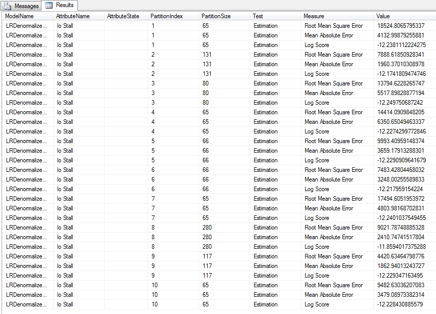
Figure 5 is an example of a Cross-Validation Report for the single Linear Regression model in a mining structure we used earlier in this tutorial series. In the bottom right corner you’ll see figures for the average value for that column in a particular model, as well as the standard deviation, which is a common measure of variability. The higher the value is, the more dissimilar the subsets of the model are from each other. If they vary substantially, that may indicate that your dataset requires more training data.[5] Figure 6 displays part of a lengthy report for one of the DecisionTrees structures we used earlier in this series, which oddly produced sets of values for just two of its five processed models, DTDenormalizedView1ModelDiscrete and DTDenormalizedView1ModelDiscrete2. The results are based on a Target Attribute of “Name” and Target State of “dm_exec_query_stats” (which together refer to the name of a table recorded in the sp_spaceused table we used for practice data) and a Target Threshold of 0.2, Fold Count of 10 and Max Cases of 1,000. In addition to Lift Score, Root Mean Square Error and Log Score we discussed above, you’ll see other measures like True Positive, which refers to the count of successful predictions for the specified attribute-value pair and probability. True Negative refers to cases in which successful predictions were made outside the specified rangers, while False Positive and False Negative refer to incorrect predictions for the same. Explanations for these measures are curiously missing from the current desktop documentation for SQL Server 2012, so your best bet is to consult the MSDN webpage Measures in the Cross-Validation Report for guidance. It also speaks of Pass and Fail measures which are not depicted here, but which refer to assignments of cases to correct and incorrect classifications respectively.
Figure 6: Cross-Validation with Classification and Likelihood Measures (click to enlarge)

Validation for Clustering models is handled a bit differently. In the dropdown list for the Target Attribute you’ll see an additional choice, #CLUSTER, which refers to the cluster number. Selecting this option returns a report like the one depicted below, which contains only measures of likelihood for each cluster. Clustering also uses a different set of DMX stored procedures than the other algorithms to produce the data depicted in cross-validation reports. The syntax for SystemGetClusterCrossValidationResults is the same as the SystemGetCrossValidationResults used by the other algorithms, except that the former does not make use of the Target State and Target Threshold parameters. The same rules that apply in the GUI must also be adhered to in the DMX Code; in Figure 8, for example, we can’t set the Target State or Target Threshold because the predictable attribute we selected has a Content type of Continuous. In both cases, we can add more than one mining model by including it in a comma-separated list. As you can see, the output is equivalent to the cross-validation reports we just discussed.
Figure 7: Cross-Validation with #CLUSTER (click to enlarge)

Figure 8: Cross-Validating a Cluster Using the Underlying DMX Stored Procedure
CALL SystemGetClusterCrossValidationResults(ClusteringDenormalizedView1Structure,ClusteringDenormalizedView1Model, ClusteringDenormalizedView1Model3,
10, – Fold Count
1000 – Max Cases
)

Figure 9: Cross-Validating Using the DMX Stored Procedure SystemGetCrossValidationResults
CALL SystemGetCrossValidationResults(
LRDenormalizedView1Structure, LRDenormalizedView1Model, – more than one model can be specified in a comma-separated list
10, – Fold Count
1000, – Max Cases
‘Io Stall’, – the predictable attribute in this case is Continuous, so we can’t set the Target State and Threshold
NULL, – Target State
NULL) – Target Threshold, i.e. minimum probability, on a scale from 0 to 1

Similarly, we can use other DMX procedures to directly retrieve the measures used to build the scatter plots and lift charts we discussed earlier. As you can see, Figure 10 shows the Root Mean Square Error, Mean Absolute Error and Log Score measures we’d expect when dealing with a Linear Regression algorithm, which is where the data in LRDenormalizedView1Model comes from. The data applies to the whole model though, which explains the absence of a Fold Count parameter. Instead, we must specify a flag that tells the model to use only the training cases, the test cases, both, or either one of these choices with a filter applied as well. In this case we’ve supplied a value of 3 to indicate use of both the training and test cases; see the TechNet webpage “SystemGetAccuracyResults (Analysis Services – Data Mining)” for the other code values. Note that these are the same options we can choose from on the Input Selection tab. I won’t bother to provide a screenshot for SystemGetClusterAccuracyResults, the corresponding stored procedure for Clustering, since the main difference is that it’s merely missing the three attribute parameters at the end of the query in Figure 10.
Figure 10: Using the SystemGetAccuracyResults Procedure to Get Scatter Plot and Lift Chart Data
CALL SystemGetAccuracyResults(
LRDenormalizedView1Structure, LRDenormalizedView1Model, – more than one model can be specified in a comma-separated list
3, – code returning both cases and content from the dataset
‘Io Stall’, – the predictable attribute in this case is Continuous, so we can’t set the Target State and Threshold
NULL, – Target State
NULL) – Target Threshold, i.e. minimum probability, on a scale from 0 to 1

These four stored procedures represent the last DMX code we hadn’t covered yet in this series. It would be child’s play to write procedures like the T-SQL scripts I provided last week to encapsulate the DMX code, so that we can import the results into relational tables. This not only allows us to slice and dice the results with greater ease using views, windowing functions, CASE statements and Multidimensional Expressions (MDX) queries in cubes, but nullifies the need to write any further DMX code, with the exception of prediction queries. There are other programmatic means of accessing SSDM data we have yet to cover, however, which satisfy some narrow use cases and fill some specific niches. In next week’s post, we’ll cover a veritable alphabet soup of additional programming tools like XMLA, SSIS, Reporting Services (RS), AMO and ADOMD.Net which can be used to supply DMX queries to an Analysis Server, or otherwise trigger some kind of functionality we’ve already covered in the GUI.
[1] See the Wikipedia page “Cross Industry Standard Process for Data Mining” at http://en.wikipedia.org/wiki/Cross_Industry_Standard_Process_for_Data_Mining
[2] See the Wikipedia page “SEMMA” at http://en.wikipedia.org/wiki/SEMMA
[3] Yet it is important to keep in mind – as many academic disciplines, which I will not name, have done in recent memory – that this says nothing about how well our dataset might compare with others. No matter how good our sampling methods are, we can never be sure what anomalies might exist in the unknown data beyond our sample. Efforts to go beyond the sampled data are not just erroneous and deceptive, but do disservice to the scientific method by trying to circumvent the whole process of empirical verification. It also defies the ex nihilo principle of logic, i.e. the common sense constraint that you can’t get something for nothing, including information content.
[4] MacLennan, Jamie; Tang, ZhaoHui and Crivat, Bogdan, 2009, Data Mining with Microsoft SQL Server 2008. Wiley Publishing: Indianapolis.
[5] IBID., p. 175.

![]()
