

In previous installments of the SQLServerCentral.com Best Practices Clinic article series, we focused on some very high-level properties of the two-node active/active SQL Server cluster that runs the back-end databases for SQLServerCentral.com and Simple-Talk.com. In this clinic, I am going to take a high-level look at some of the key performance counters for each instance and see if we can identify any potential bottlenecks.
To help me identify potential bottlenecks, and for you to follow along if you wish, I am going to use the live version of SQL Monitor that you can view at monitor.red-gate.com. This live version monitors both instances on a real-time, as well as a historical, basis: This makes it easy for me to quickly identify any potential resource bottlenecks on either instance. If you decide to follow along, keep in mind that the performance counter graphs that I show here will probably be different from the ones you see when you check out the live version of SQL Monitor, because performance data is dynamic, and the 24-hour snapshot of the counters that I discuss in this article will vary over time.
Checking Out Key Performance Monitor Counters
If you are not familiar with SQL Monitor, I’d better mention that it includes several different ways to check on the health of SQL Server instances. For this particular article, I am going to focus exclusively on the “Analysis” screen, which allows me to view a wide variety of Performance Monitor counters over various time spans. This screen allows me to view performance counter data for one or the other of the two instances, or I can view both at the same time on the same screen.
SQL Monitor collects twenty-seven key performance counters. I’m not going to check out all of them, but instead focus on those seven counters that can help me determine if there might be potential resource bottleneck on either of the two instances. The counters I am going to examine include:
CPU
- Machine: Processor Time (Processor: % Processor Time (_Total)
- Average CPU Queue Length (System: Processor Queue Length / Number of Logical Processors)
Memory
- Machine: Memory Used (Total Server Memory – Memory: Available Bytes)
- Buffer Free Pages (Buffer Manager: Free Pages)
IO
- Disk Average Read Time (Logical Disk: Average Disk Sec/Read)
- Disk Average Write Time (Logical Disk: Average Disk Sec/Write)
Network
- Network Utilization (8 * ((Network Interface: Bytes Received/sec) + (Network Interface: Bytes Sent/sec)) / (Network Interface: Current Bandwidth) *100)
You’ll have noticed that some of the names used for performance counters in SQL Monitor are different from those used in Performance Monitor. Whereas some of the SQL Monitor counters such as ‘Disk Average Read Time = Logical Disk: Average Disk Sec/Read’ correspond exactly with Performance Monitor counters, other SQL Monitor counters are derived from Performance Monitor counters; For example, ‘Average CPU Queue Length’ is equivalent to ‘System: Processor Queue Length / Number of Logical Processors’. This has been done to make it easier to fully understand what is going on inside your SQL Server instance. For the purposes of this article, I will be using the SQL Monitor terminology.
As you probably know, you don’t get enough information from looking at these performance counters by themselves, without any context, to make any hard conclusions about resource bottlenecks. You’ll also need to dip into the wealth of additional information that SQL Server provides by such means as DMOs (Dynamic Management Objects) before you can make any definitive conclusions. But for the purposes of this article, I am going to focus exclusively on performance counters, as this is the easiest for me to talk about, and at the same time, allows you to follow along by using the live version of SQL Monitor.
Selecting a Time Range for Analysis
SQL Monitor allows you to look at performance counter data over a wide variety of time frames, from as little as 10 seconds, to as long as you have data stored (typically one week). One thing to keep in mind when viewing performance counter statistics is that the longer the time scale, the less detailed the data; the shorter the time frame, the more detailed the statistics. In other words, longer time ranges tend to hide spikes of data, showing you more average values, while shorter time ranges show more spikes, as data is averaged over a shorter period of time.
There are pros and cons of using both longer and shorter time periods. Longer time periods are good for identifying trends, while shorter time periods are better for seeing in detail exactly what is happening at a particular point in time. Often, when I am examining performance counters on a SQL Server instance, I will begin by looking at longer time ranges and, if I find anything of interest, I will then drill down into narrower time periods in order to find out exactly what is going on.
I don’t have time in this article to look at a lot of different time periods, so I have decided to focus on a typical 24 hour weekday, starting at midnight. This gives me a good feel for any kinds of cycles an instance might be experiencing over a typical day.
So let’s take a look at the seven performance counters to see if we can identify any potential resource bottlenecks in the two SQL Server instances running SQLServerCentral.com and Simple-Talk.com.
Note: Both servers have identically configured hardware, so any differences in performance between the two servers can’t be attributed to differences in hardware.
Looking for Potential CPU Bottlenecks
To help identify any potential CPU bottlenecks on the two SQL Server instances, I am going to look at both ‘Machine: Processor Time’ and ‘Average CPU Queue Length’. To start out, let’s look at these two counters for both of these instances over a typical 24 hour day.
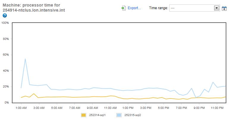
Figure 1: Machine: Processor Time for both instances over 24 hours.
Let’s start with one of the most common CPU resource indicators available to us, and that is ‘Machine: Processor Time’, which shows the total CPU utilization of all the cores for each of our instances. Each server has two, four-core CPUs (without hyperthreading), or a total of eight cores per server.
In figure 1, the yellow line represents the Simple-Talk.com server, and it is fairly obvious that the CPU utilization for the Simple-Talk server is well below any potential bottleneck threshold. In fact, you could say this server was underutilized, at least from a CPU perspective during the 24 hours this graph represents.
The blue line represents the SQLServerCentral.com server, and while the overall CPU utilization is higher than the Simple-Talk server, it is still not a very busy server. The busiest time of the day peaks at about 55% CPU utilization at 1:27 AM. This is during the time frame that the SQLServerCentral.com server is creating and emailing over 800,000 newsletters, which generally occurs between 10:00 PM and 4:00 AM daily (notice that the CPU runs higher than normal during this time frame). I know from previous experience with this server that there are a number of inefficient queries used for the mailing job, which need some tuning. But even without any tuning, there is no CPU bottleneck to worry about, as 55% CPU utilization does not indicate a problem.
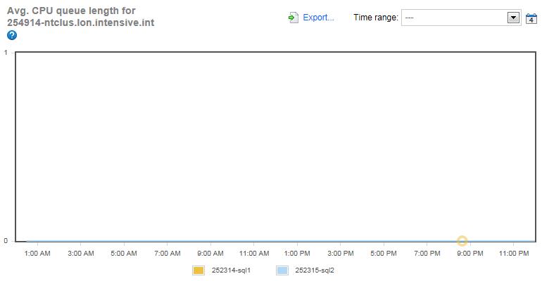
Figure 2: Average CPU Queue Length for both instances over 24 hours.
The fact that there are no CPU bottlenecks on these two servers is further reinforced by examining the Average CPU Queue Length for each server. This counter gives an indication of how many CPU requests are stacked up waiting to be executed. The higher the queue length, the greater the likelihood of a CPU bottleneck. As you can see in figure 2, this counter is zero for the entire 24 hour time period, indicating that there are no CPU bottlenecks.
It is very likely that, if you examine the data for both of these counters at a finer level such as at a one hour time-frame instead of a 24 hour time-frame, you will see more and higher spikes. This is because the data in these graphs are averaged over 24 hours and will not show all the spikes that occur minute-by-minute. In most cases, it is better for our purpose that occasional spikes are averaged out over the 24 hour graph, as DBAs are generally more interested in overall trends, and not specific incidents of high CPU activity. Of course, if you do want to drill down and see very specific activity, you can easily do so using SQL Monitor.
So based on both of the above counters, it appears that neither SQL Server instance is experiencing any CPU-related bottlenecks.
Looking for Potential Memory Bottlenecks
Memory is area where bottlenecks can often happen in memory usage, and so I’ll be looking at two different counters to see what is going on with these two instances. They include: ‘Machine: Memory Used’ and ‘Buffer Free Pages’. Let’s look at these two counters for both of these instances over a typical 24 hour day. For reference, each server has 24 GB of RAM memory.
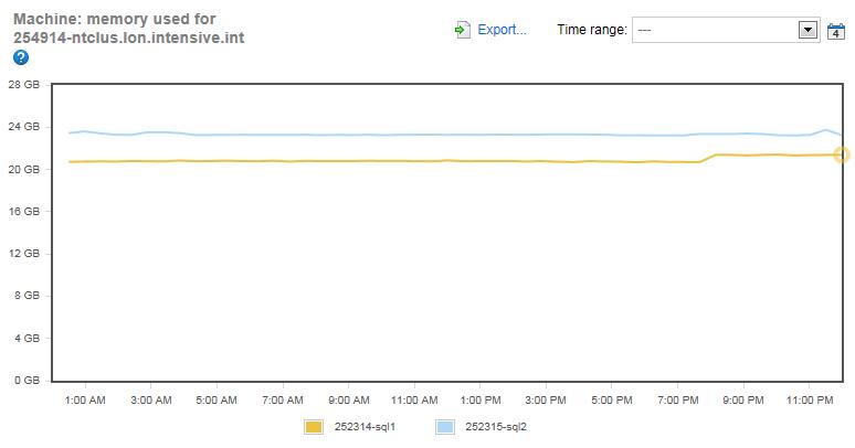
Figure 3: Machine: Memory Used for both instances over 24 hours.
The yellow line, which represents the Simple-Talk server, indicates that the entire system is using between 20 and 21 GB of RAM. Given that the server has 24 GB of available RAM, this indicates that the server has more than enough RAM to run, otherwise it could request more and get it. On the other hand, the blue line, which represents SQLServerCentral.com, is using virtually the entire available RAM, indicating a potential memory bottleneck. Of course, it isn’t sufficient to look at just this single before making any judgments about memory bottlenecks.
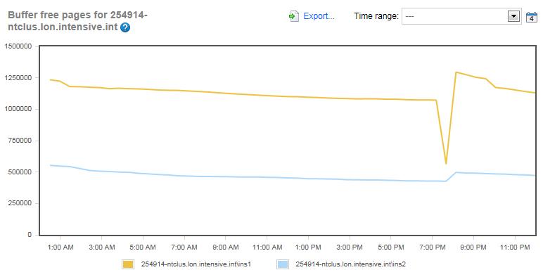
Figure 4: Buffer Free Pages for both instances over 24 hours.
The ‘Buffer Free Pages’ counter measures how many free buffer pages are available in the buffer cache. The fewer the number of free pages available in the buffer cache, the more likely the server might be under memory-pressure and experiencing a memory bottleneck. Unlike the ‘Machine: Memory Used’ graph, this graph has substantially more variation. If you look closely at the graph, you will see that, at even at the lowest number of available free pages, which is 426,752 for the blue line, this is still a huge number of available free buffer cache pages that are not being used. This would appear to indicate that both SQL Server instances have more than enough free pages available should more be needed. In turn, this seems to indicate that memory is not a bottleneck in either server.
As you look at figure 4, you will notice that both servers had a drop in Buffer Free Pages at 7:40 PM. Given the coincidence that both servers have their lowest Buffer Free Pages of the day at the same time, do you have any idea what might be causing this? If you guessed ‘database maintenance’, then you are right. It is at this time, each day, that the indexes are rebuilt and the DBCC CHECKDB commands are run on each server. As these commands run, more data has to be read into the buffer cache so that the number of available Buffer Free pages drops, but as you can see that, once the maintenance stops, both servers return to normal fairly quickly.
So are there any memory bottlenecks on these two servers? I think it is clear that the Simple-Talk server doesn’t have any memory-pressure. On the other hand, the SQLServerCentral.com server is a little tougher to call using only these two performance counters. I say this because virtually the entire RAM in the server is being used, which is a warning flag to me. Because the counters are not as clear cut for the SQLServerCentral.com server as the Simple-Talk server, I think that memory usage in the SQLServerCentral.com server warrants additional investigation with other tools. In the next section, when we talk about IO counters, we will see another hint that perhaps indicates memory-pressure on the SQLServerCentral.com server.
Looking for Potential IO Bottlenecks
Disk IO bottlenecks are a common problem in most SQL Servers, and we will be using two performance counters to help us determine if there are any potential IO bottlenecks on our two servers: ‘Disk Average Read time’ and ‘Disk Average Write Time’. These two counters measure disk latency. Generally when I look at disk read and write-latency, I use the following chart to guide me as to whether or not an IO bottleneck might be a problem.
- Less than 10 milliseconds (ms) = very good
- Between 10-20 ms = okay
- Between 20-50 ms = slow
- Greater than 50-100 ms = potentially serious IO bottleneck
- Greater than 100 ms = definite IO bottleneck
Keep in mind that these are very generic numbers and should be used only as loose guidelines, as each environment is different.
Before we begin looking for potential IO bottlenecks, you first need to know a little about how the drives are configured for each instance.
Simple-Talk.com:
- V: MDF files (Dedicated RAID 10 SAN array)
- W: LDF files (Dedicated RAID 10 SAN array)
- X: TEMPDB (Dedicated Mirrored array on SAN)
SQLServerCentral.com:
- S: MDF files (Dedicated RAID 10 SAN array)
- T: LDF files (Dedicated RAID 10 SAN array)
- U: TEMPDB (Dedicated Mirrored array on SAN)
Unlike the CPU-related counters, where I combine the counters of both SQL Server instances on the same screen, I am going to separate them in this example, as doing so makes it easier to read the graphs.
Simple-Talk Disk IO Latency
Now that you know a little about how the data is distributed on the two servers, let’s take a look at the disk latency for the three key Simple-Talk.com arrays and see if there are any IO bottlenecks throughout our 24 hour period.
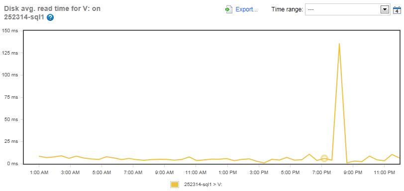
Figure 5: The Disk Average Read Time for the MDF files on the Simple-Talk Server (Drive V:).
For most of the day, the Disk Average Read Time for the MDF files on the Simple-Talk server was less than 10 ms, which is very good performance. The only time when a read bottleneck occurred was during the maintenance window, when it peaked at 135 ms for a short time.

Figure 6: The Disk Average Write Time for the MDF files for the Simple-Talk server (Drive V:)
The write-latency for the same drive averaged about 10 ms for most of the day, except when it peaked at about 54 ms, which was about the same time as the read time peaked during the maintenance window.
Overall, I am happy with the read and write disk latency of the Simple-Talk.com MDF array, as it typically ran 10 ms or less for reads and writes, other than during the maintenance window, where higher than average activity is to be expected. On the other hand, it might be possible to tweak the maintenance work in order to reduce some of the maintenance load. I’ll look at the Simple-Talk.com and the SQLServerCentral.com maintenance jobs in a future clinic article to see if any improvements can be made in them.

Figure 7: The Disk Average Read Time for the LDF files for the Simple-Talk server (Drive W:).
The array with the LDF files for Simple-Talk.com has very low read latency, typically under 10 ms. As might be expected, there was a peak during the maintenance window, but it only peaked at about 32 ms. I also want to mention that transactional replication is turned on for this server, and that the log file of one of the databases on this server is being read by the Log Reader Agent, which can contribute to a slightly higher than typical read-latency for the LDF array. But as you can see, it is insignificant.
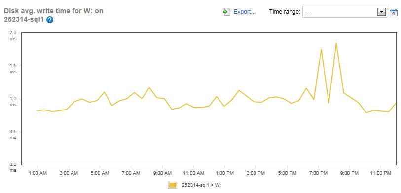
Figure 8: The Disk Average Write Time for the LDF files for the Simple-Talk server (Drive W:).
The same goes for the write-latency for the LDF array, which kept to around 1 ms throughout the day, with only a slight increase during the maintenance period.
Both the read and write-latency of the LDF drive array for the Simple-Talk.com server are very good and show no signs of any IO bottlenecks.

Figure 9: The Disk Average Read Time for the TEMPDB files for the Simple-Talk server (Drive X:).
The mirrored array dedicated to TEMPDB averaged a read-latency of between 1-2 ms most of the time for the Simple-Talk.com server, with only a few peaks of around 6 ms, which is great performance.
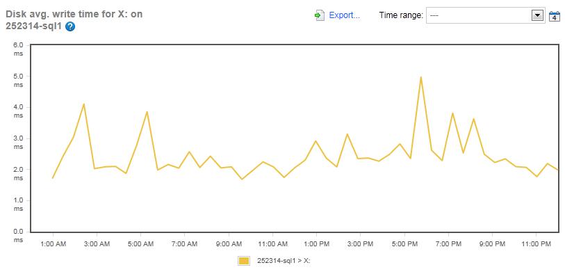
Figure 10: The Disk Average Write Time for the TEMPDB files for the Simple-Talk server (Drive X:).
Like the read-latency of the TEMPDB, the write-latency was minimal throughout the day, averaging about 5ms. I think that it is very clear from these figures that there is no IO bottleneck in the TEMPDB array for the Simple-Talk.com server.
Now let’s take a look at the SQLServerCentral.com server and see what its IO performance was like.
SQLServerCentral.com Disk IO Latency>
Let’s see if the SQLServerCentral.com server has any IO bottlenecks. As with the Simple-Talk.com server, we will look at three arrays, one for the MDF files, one for the LDF files, and one for TEMPDB.
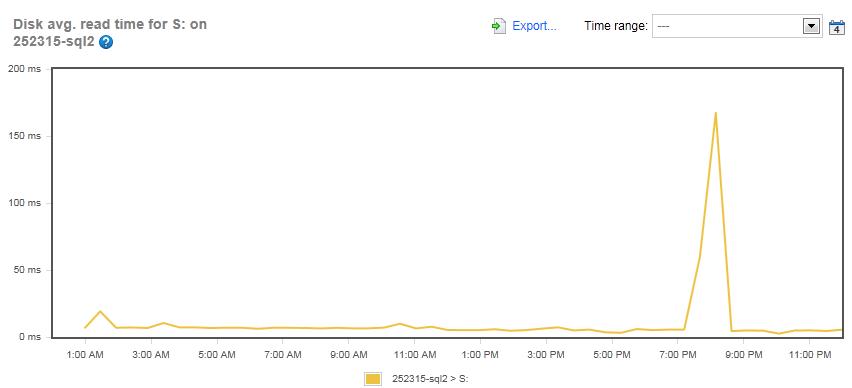
Figure 11: The Disk Average Read Time for the MDF array on the SQLServerCentral.com server (Drive S:)
The read-latency for the MDF array on SQLServerCentral.com looks almost identical to the Simple-Talk server, with an average of less than 10 ms, and a peak of 167 ms during the maintenance period.
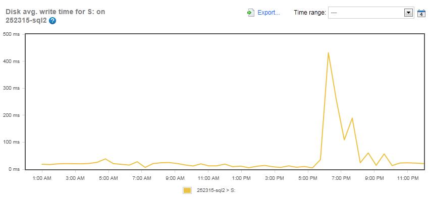
Figure 12: The Disk Average Write Time for the MDF array on the SQLServerCentral.com server (Drive S:)
Now, things begin to change when it comes to write-latency for the MDF array on the SQLServerCentral.com server. If you look closely at figure 12, the scale on the Y-axis is quite different than the one in figure 11. For most of the day, write-latency averaged about 20 ms, which is a little on the high side; but for about a 3-4 hour windows in the evening, write-latency spiked greatly, peaking at 431 ms (in the middle of the maintenance window). This high latency tells me that there is a definite IO bottleneck within this 3-4 hour window.
So what might account for the relatively high write-latency for this MDF array? Based on my knowledge of this server, there are a number of factors that may be involved. These include:
- It’s a busy server with more databases, and larger databases, than the Simple-Talk.com server.
- The bigger the databases, the more resources the maintenance job uses.
- The SQLServerCentral.com server is used to help produce a daily newsletter, and this job runs from 10:00 PM to about 4:00 AM every night. This doesn’t seem to add a lot of extra writes, but you can see that this time range does show an overall increase in disk latency.
Each of the above reasons contributes to the additional work the server has to do, which may account for the higher write-latency of the server. But is increased work the only reason? Think back to the memory counters we looked at earlier. Remember that the SQLServerCentral.com server is using all of the available RAM. One explanation of the higher write-latency might be that the server is under memory-pressure and has to write out to disk more often. In fact, I think that, based on the data we have already, the memory-pressure problem might be a good working hypothesis as to why disk latency is high on this array. Of course, to find out, we need to look at additional information about the server to see if this is really the case. And if it is, then it might be justifiable to add more RAM to the server, which would allow more data to be cached, and in return, helping to reduce write-latency. I’ll follow up on this hypothesis in a later clinic article.
But for now let’s check the LDF array to see if it is experiencing the same type of IO bottleneck as the MDF array.

Figure 13: The Disk Average Read Time for the LDF array on the SQLServerCentral.com server (Drive T:)
Right away, you can see that the read-latency on the LDF array of the SQLServerCentral.com server is high. In fact, the average for the 24 hour period is 32.4 ms, well into the slow area of disk latency, indicating a potential bottleneck. This is especially worrisome as LDF files should generally only be written to, not read from, most of the time. In other words, what is causing all of the reads on these LDF files? This needs some follow-up investigation to see exactly what is going on. I hope to do this in a future clinic article. So, is there also an IO problem with writes to the LDF files? Let’s find out.
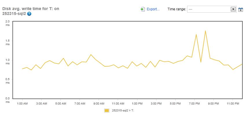
Figure 14: The Disk Average Write Time for the LDF array on the SQLServerCentral.com server (Drive T:)
This is good news. The write-latency over the 24 hour period averages just .9 ms, which is a great number, with a peak of only 1.8 ms during the maintenance window. So this means that whatever is causing the read-latency is not contributing to write-latency. This makes me feel a little better, as write-latency of LDF files is critical to the overall performance of an instance. This is because all data modifica
Now, let’s check on the read and write-latency of TEMPDB.

Figure 15: The Disk Average Read Time for the TEMPDB array on the SQLServerCentral.com server (Drive U:)
Right away, we can see that the read-latency averages just over 1 ms for most of the day, and only peaks at 3.5 ms during the maintenance window.
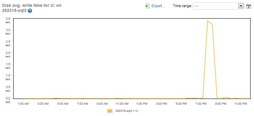
Figure 16: The Disk Average Write Time for the TEMPDB array on the SQLServerCentral.com server (Drive U:)
And when we look at the write-latency for the TEMPDB array, we see that it is virtually zero most of the day, with only a spike of 3.5 ms during the maintenance window. Based on these last two graphs, I think we can easily conclude that the TEMPDB array does not have any IO-related problems.
So where does this leave us, now that we have examined the read and write-latency for the SQLServerCentral.com MDF, LDF, and TEMPDB arrays? We seem to have potential problems in the write-latency of the MDF array and in the read-latency of the LDF array. In the bigger picture of all the drives, these don’t seem like a huge problem, and it is possible even if we can improve the latencies in these two areas that the end users (those of you who visit SQLServerCentral.com) would even notice. I definitely think we need to follow up on these two areas to see what is happening and consider whether there are any explanations or easy fixes.
Looking for Potential Network Bottlenecks
Based on my experience, the network connection between your SQL Servers and their clients is the least likely area to see a bottleneck, especially if you are using 1Gbs network cards and switches. Of course, there are always exceptions and you should look for potential network bottlenecks, even though they are unlikely.
The counter used by SQL Monitor to track network performance is called Network Utilization, and it is a derived counter. By this, I mean the data it returns is not exactly like the data you would get from similar Performance Monitor counters. Instead, it performs a little calculation and makes it very easy to see how much of the bandwidth of a particular SQL Server is being used. So let’s take a look at our two instances and see if we have any potential bottlenecks.

Figure 17: Network Utilization for Simple-Talk.com server.
For most of the day, network utilization for the Simple-Talk server runs about 4%, but there are two spikes. The large spike, 80% at 1:27 AM, is a result of backups being copied over the network to and from this server. What happens is that when backups are made on the Simple-Talk server, they are simultaneously made over the network onto the SQLServerCentral.com server, for additional redundancy of backups. In turn, and at about the same time, backups on the SQLServerCentral.com server are copied over the network to the Simple-Talk server. This results in a lot of network traffic, causing the spike we see in figure 17. This problem could be alleviated by scheduling the backups on each server slightly differently, and I will be taking a look at why the backups have been configured this way, and see if they can be scheduled slightly differently so as to spread out the network traffic load.
The small spike of 12% at about 8:00 PM occurs about the time of the maintenance window. Overall, I would consider network utilization not to be a problem with the Simple-Talk server.
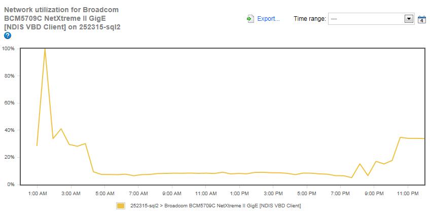
Figure 18: Network Utilization for SQLServerCentral.com server.
The typical network utilization for the SQLServerCentral.com server runs about 8% most of the day, but there is a very large spike that reaches 100% at 1:27 AM, the same time the network utilization peaks on the Simple-Talk.com server. As previously discussed, this is when backups are copied back and forth over the network. There is a lot of network activity between 10:00 PM and 4:00AM on the server as well. This is network traffic that is generated by the newsletter creation process. Adding both the backup and newsletter creation traffic at the same time, we see that the network utilization becomes bottlenecked.
I am going to investigate why both of these network intensive tasks are scheduled to overlap and see if it is possible to reduce the overlapping of activity to prevent this temporary bottleneck. On the other hand, this is occurring at night, so it is doubtful any users are affected by this temporary bottleneck, but it is still worth investigating.
So What Did We Find Out?
By just checking out seven different performance counters over a 24 hour period on two different instances, we were able to determine that the Simple-Talk server does not appear to be experiencing any resource bottlenecks. On the other hand, we discovered that the SQLServerCentral.com server may be experiencing memory, IO, and network bottlenecks at various times of the day. In order to better determine what is causing these problems, and how to fix them, will take additional work. In future clinics, I intend to delve deeper into these servers, taking a more in-depth look at them using a variety of different tools.
It would be really interesting to hear your comments on the series so far, hit the 'join the discussion' bottom below to add your feedback.