

Since “the generation of random numbers is too important to leave to chance” (quoting Robert R. Coveyou of the Oak Ridge National Laboratory), we would like to take just a smidgen of your valuable time to build on the work of SQL MVP Jeff Moden and others, regarding the generation of random numbers using SQL. Specifically we would like to examine some techniques to generate non-uniformly distributed random numbers (NURN) from uniformly distributed random numbers (URN); including a few basic statistical distributions to get you started.
As we all know, random numbers have important uses in simulations (specifically Monte-Carlo simulations), cryptography and many other highly technical fields, in addition to having utility in generating large quantities of random data for testing the performance of our SQL endeavors.
Since I am certainly no statistician, we will only empirically examine the apparent randomness of the resulting random numbers generated by SQL, without delving deeply into the mathematics of how to test whether pseudo random numbers are truly random or merely appear to be so. Our intent will be to show correctness of the implementation of the algorithms we will employ and to demonstrate whether the resulting random number streams are likely to be good enough to use for non-critical purposes.
The general technique for transforming a URN into a NURN is to multiply the URN by the inverse of the cumulative distribution function (CDF) for the target distribution. In practice, this is technically challenging for many distributions that do not have a computationally efficient method of evaluating the CDF or for those where the CDF does not exist in a closed analytical form. Fortunately those much wiser than us have analyzed various distributions and have come up with approximations that will suit our needs in many cases.
The Test Harness
In our test harness we have constructed calls to our various NURN generators by creating a pseudo URN of type FLOAT using standard SQL techniques and then passing it to a transformation FUNCTION. We will consistently employ Scalar Valued Functions including WITH SCHEMABINDING for performance reasons, however in practice you may want to test equivalent in-line Table Valued Functions where possible to see if performance can be improved. First we will set up some test data.
-- Data definition and setup
DECLARE @NumberOfRNs   INT
       ,@Lambda        FLOAT     -- For the Poisson NURNs
       ,@GaussianMean  FLOAT     -- For the Normal NURNs
       ,@GaussianSTDEV FLOAT
       ,@LambdaEXP     FLOAT     -- For the Exponential NURNs
       ,@WeibullAlpha  FLOAT     -- For the Weibull NURNs
       ,@WeibullBeta   FLOAT
       ,@Laplaceu      FLOAT     -- For the Laplace NURNs
       ,@Laplaceb      FLOAT
SELECT @NumberOfRNs    = 1000000
      ,@Lambda         = 4.0     -- Lambda for the Poisson Distribution
      ,@GaussianMean   = 5       -- Mean for the Normal Distribution
      ,@GaussianSTDEV  = 1.5     -- Standard Deviation for the Normal Distribution
      ,@LambdaEXP      = 1.5     -- Lambda for the Exponential Distribution
      ,@WeibullAlpha   = 1.0     -- Alpha (scale) for the Weibull Distribution
      ,@WeibullBeta    = 1.5     -- Beta (shape) for the Weibull Distribution
      ,@Laplaceu       = 4.0     -- Mu (location) for the Laplace Distribution
      ,@Laplaceb       = 1.0     -- Beta (scale) for the Laplace Distribution
--CREATE TYPE Distribution AS TABLE (EventID INT, EventProb FLOAT, CumProb FLOAT)
DECLARE @Binomial      AS Distribution
    ,@DUniform         AS Distribution
    ,@Multinomial      AS Distribution
-- Simulate a coin toss with a Binomial Distribution
INSERT INTO @Binomial
SELECT 0, 0.5, 0.5 UNION ALL SELECT 1, 0.5, 1.0
-- Events returned by this Discrete Uniform distribution are the 6
-- Fibonacci numbers starting with the second occurrence of 1
INSERT INTO @DUniform
SELECT 1, 1./6., 1./6. UNION ALL SELECT 2, 1./6., 2./6.
UNION ALL SELECT 3, 1./6., 3./6. UNION ALL SELECT 5, 1./6., 4./6.
UNION ALL SELECT 8, 1./6., 5./6. UNION ALL SELECT 13, 1./6., 1.
-- Events returned by this Multinomial distribution are the 5
-- Mersenne primes discovered in 1952 by Raphael M. Robinson
INSERT INTO @Multinomial
SELECT 521, .10, .10 UNION ALL SELECT 607, .25, .35 UNION ALL SELECT 1279, .30, .65
UNION ALL SELECT 2203, .15, .80 UNION ALL SELECT 2281, .2, 1.
Here is the test harness, for generating the NURNs for our target distributions:
-- Create random numbers for the selected distributions
SELECT TOP (@NumberOfRNs)
     RandomUniform     = URN
    --,RandomPoisson     = dbo.RN_POISSON(@Lambda, URN)
    ,RandomBinomial    = dbo.RN_MULTINOMIAL(@Binomial, URN)
    ,RandomDUniform    = dbo.RN_MULTINOMIAL(@DUniform, URN)
    ,RandomMultinomial = dbo.RN_MULTINOMIAL(@Multinomial, URN)
    ,RandomNormal      = dbo.RN_NORMAL(@GaussianMean, @GaussianSTDEV, URN, RAND(CHECKSUM(NEWID())))
    ,RandomExponential = dbo.RN_EXPONENTIAL(@LambdaEXP, URN)
    ,RandomWeibull     = dbo.RN_WEIBULL(@WeibullAlpha, @WeibullBeta, URN)
    ,RandomLaplace     = dbo.RN_LAPLACE(@Laplaceu, @Laplaceb, URN)
 INTO #MyRandomNumbers
 FROM sys.all_columns a1 CROSS APPLY sys.all_columns a2
 CROSS APPLY (SELECT RAND(CHECKSUM(NEWID()))) URN(URN)
In later sections, we will describe each distribution in turn, but let’s clear up a few basic questions right now about the test harness.
- The algorithm employed to generate Gaussian distributed NURNs requires two URNs.
- We use our RN_MULTINOMIAL FUNCTION to generate three different distributions because it is a more general case of the other two (further explanation will be provided in that section).
- It is necessary to CREATE the TYPE prior to CREATE FUNCTION RN_MULTINOMIAL, because this object is used in that FUNCTION. The TYPE object was introduced in SQL Server 2008 and that is the only issue that prevents these solutions being used in SQL Server 2005 – the alternative being that you could pass the table using XML.
- We have attached two SQL scripts to run the examples from: 1) Setup FUNCTIONs.sql (run this first) and 2) Generate NURNs.sql (takes about 4.5 minutes to run with 1,000,000 random numbers generated. The latter also contains some commented out DROPs at the end for cleanup of your sandbox.
Uniform Random Numbers – How Uniform?
Since all of our follow up distributions are based on generating URNs, we’ll take a quick look at how uniform these numbers are when generated by the standard SQL construct. If the uniformity of these numbers is skewed in any way, it will have a corresponding impact on all of the remaining distributions.
The mean of a sample of uniform random numbers on the interval {0, 1} is simply 0.5. The variance for this same interval is 1/12. For our sample of 1,000,000 URNs, we got these results using the SQL AVG() and VAR() built-in functions. These results are reasonably close to expectations.
PopulationMean PopulationVAR SampleMean SampleVAR
4 0.083333 0.499650832838227 0.0832923192890653
A histogram of our URNs is useful to see how well behaved they are across some pre-defined intervals.

The results show, in our opinion that the uniformity is not great but probably good enough for noncritical purposes. Note that we did this run many times and looked at many results, each slightly different and these results were not specially selected. When you run our SQL yourself, your results will be different.
Multinomial Random Numbers
Before we discuss the Multinomial distribution, let us first quickly mention two other discrete distributions.
The Binomial distribution is most widely understood in the context of modeling the flip of a coin. It expresses the probability of the occurrence of a binary event (heads or tails), returning either a 0 or a 1 (or other N) to indicate whether or not that event occurred (this can also be thought of as “success” or “failure”). Of course, a fair coin toss would return 50% heads and 50% tails, however the Binomial distribution allows for other probabilities besides 50% because life isn’t always fair.
The Discrete Uniform distribution describes a series of events (more than 2), such as the roll of a dice, where the probability of each specific event is identical. Of course, this is similar to the method of generating random integers based on a range and offset described by Jeff Moden here.
The Multinomial distribution is a more general case of the two. It models a series of events where the probability of the occurrence of each event may be different.
Remember of course that events don’t need to be a simple set of integers like 0, 1, 2, … n. They could be anything (including negative integers). For example, in our setup for the Multinomial distribution we have chosen our events be the five Mersenne primes discovered by Raphael M. Robinson in 1952, and for our Discrete Uniform distribution they are the first six Fibonacci numbers starting with the second occurrence of 1. These events could also be FLOATs by changing the data type of EventID in the Distribution TYPE to FLOAT.
If we look at the three table variables we set up in our test harness, we can see that:
- @Binomial defines two events (0, 1) where the probability (p) of success (1) occurring is 50% and the probability of failure (0) is 1-p.
- @DUniform defines six events (1, 2, 3, 5, 8, 13) such as the roll of a dice, where the probability of any event occurring is 1/6.
- @Multinomial defines 5 events (521, 607, 1279, 2203, 2281) that may occur with different probabilities.
CREATE FUNCTION dbo.RN_MULTINOMIAL
    (@Multinomial Distribution READONLY, @URN FLOAT)
 RETURNS INT --Cannot use WITH SCHEMABINDING
AS
BEGIN
    RETURN
        ISNULL(
            (   SELECT TOP 1 EventID
                FROM @Multinomial
                WHERE @URN < CumProb
                ORDER BY CumProb)
            -- Handle unlikely case where URN = exactly 1.0
            ,(  SELECT MAX(EventID)
                FROM @Multinomial))
END
For each of our distributions, we will compare the percentage of random numbers that fall into the associated probability range.
RandomBinomial BinomialFreq EventProb ActPercentOfEvents
0 499778 0.5 0.499778000000
1 500222 0.5 0.500222000000
RandomDUniform DUniformFreq EventProb ActPercentOfEvents
1 166288 0.166666 0.166288000000
2 166620 0.166666 0.166620000000
3 166870 0.166666 0.166870000000
5 166539 0.166666 0.166539000000
8 166693 0.166666 0.166693000000
13 166990 0.166666 0.166990000000
RandomMultinomial MultinomialFreq EventProb ActPercentOfEvents
521 99719 0.1 0.099719000000
607 249706 0.25 0.249706000000
1279 300376 0.3 0.300376000000
2203 149633 0.15 0.149633000000
2281 200566 0.2 0.200566000000
Notice that across the board, the generated NURNs conform closely to the expected probabilities.
Gaussian (or Normally) Distributed Random Numbers
In a recent discussion thread, one of the SSC forum members (GPO) posted a question regarding how to generate random numbers based on a Gaussian (Normal) distribution. For his benefit I researched the question (in fact it was the inspiration for this article) and came up with the Box-Muller transform method, upon which my RN_GAUSSIAN FUNCTION is based. You can disregard my incorrect statement in that thread on how NURNs are generated from URNs.
The Gaussian distribution is a continuous distribution, probably requiring little explanation as it should be quite familiar to most of us, and it is routinely employed to analyze “normal” samples that fall regularly around a mean.
In addition to the mean, it is necessary to specify the standard deviation, to emulate the shape of the normal distribution that applies to the population being sampled.
CREATE FUNCTION dbo.RN_NORMAL
    (@Mean FLOAT, @StDev FLOAT, @URN1 FLOAT, @URN2 FLOAT)
 RETURNS FLOAT WITH SCHEMABINDING
AS
BEGIN
    -- Based on the Box-Muller Transform
    RETURN (@StDev * SQRT(-2 * LOG(@URN1))*COS(2*ACOS(-1.)*@URN2)) + @Mean
END
First we will compare the population (expected) mean and variance vs. the sample mean and variance and see a very close correspondence of the sample to the expectation.
PopulationMean PopulationSTDEV SampleMean SampleSTDEV
5 1.5 5.00049965700704 1.50020497041145
Next, we’ll take a look at a histogram of the frequency of occurrence within a series of selected, uniform intervals that is within plus or minus 3 standard deviations of the mean.

Readers familiar with the Normal distribution will immediately recognize how “normal” this sample of numbers appears! We also found that 998,596 of our 1,000,000 (99.86%) random numbers appear within 3 standard deviations of our mean, which also corresponds quite closely to statistically expected norms.
Exponential Random Numbers
The Exponential distribution is a reasonably well-behaved distribution with a CDF that can easily be described in a closed analytical form. Applications for the Exponential distribution appear in physics, hydrology, reliability theory and queuing theory.
CREATE FUNCTION dbo.RN_EXPONENTIAL (@Lambda FLOAT, @URN FLOAT)
 RETURNS FLOAT WITH SCHEMABINDING
AS
BEGIN
    RETURN -LOG(@URN)/@Lambda
END
Knowing that the population mean is 1/Lambda and the sample standard deviation is 1/Lambda^2, we can compare against our sample mean and variance and see a very close correspondence.
PopulationMean PopulationVAR SampleMean SampleVAR
0.6667 0.4444 0.666 0.4444
We can also compare the frequency distribution against a standard probability density curve obtained from the provided wiki link to confirm that the sample appears to be quite well aligned to what would be expected where Lambda = 1.5 (the light blue line).

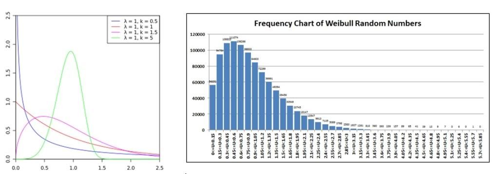
Weibull Random Numbers
Having worked with the Weibull distribution in university, even going so far as doing a derivation of the Maximum Likelihood Estimator (MLE) for it, my understanding is that it is also quite well-behaved so was a prime candidate distribution for this excursion into NURNs. The Weibull has application in many areas of statistics and engineering, including weather forecasting, survival analysis, insurance, hydrology, reliability engineering (here’s hoping that my professor for that course would be proud) and many others.
The method of generating Weibull random numbers, which can be found in the wiki link provided, is quite simple to implement as demonstrated in the RN_WEIBULL FUNCTION. The Weibull is described by a shape parameter (@WeibullAlpha in the test harness) and scale parameter (@WeibullBeta) .
CREATE FUNCTION dbo.RN_WEIBULL (@Alpha FLOAT, @Beta FLOAT, @URN FLOAT)
 RETURNS FLOAT WITH SCHEMABINDING
AS
BEGIN
    RETURN POWER((-1. / @Alpha) * LOG(1. - @URN), 1./@Beta)
END
The mean and standard deviation of a Weibull distribution are not easily calculated as they use the Gamma distribution in analytical form. So we will settle for a comparison against the wiki probability density function where the shape parameter is 1.0 and the scale parameter is 1.5 (the purple line).
Laplace Random Numbers
Either because I was a geek or because I had a great professor for this in university, I really enjoyed my Laplace transforms course. So when I learned that Laplace also described a statistical distribution, I simply had to include it in this article to pay homage to them both.
The Laplace distribution is a continuous distribution that, fortunately for us, has a relatively simple to understand CDF, and has applications in statistics and speech recognition. It is described by a location parameter (the Greek letter mu or @Laplaceu in our test harness) and a scale parameter (b or @Laplaceb).
CREATE FUNCTION dbo.RN_LAPLACE (@u FLOAT, @b FLOAT, @URN FLOAT)
 RETURNS FLOAT WITH SCHEMABINDING
AS
BEGIN
    RETURN @u - @b * LOG(1 - 2 * ABS(@URN - 0.5)) *
        CASE WHEN 0 < @URN - 0.5 THEN 1
             WHEN 0 > @URN - 0.5 THEN -1
             ELSE 0
        END
END
The Laplace distribution has an easy to calculate mean (@Laplaceu) and standard deviation (2*@Laplaceb^2), so once again we will compare the results of our population vs. sample.
PopulationMean PopulationVAR SampleMean SampleVAR
4 2 4.0009 1.9975
We will once again compare the wiki probability density function (mu=0, b=1, i.e., the red line) against a histogram of our sample. In our case, we used 4.0 for our location parameter, changing only where the peak probability clusters (around 4 instead of 0).

Conclusions
Our conclusion from these studies is that the implementation of our NURN generators appears to be correct, at least when compared empirically against standard histograms published for such distributions. Furthermore, in general we see a close correspondence between population mean and standard deviation (or variance), or otherwise to the expected probability for each discrete event. All of our sample results are included in the attached Excel worksheet.
In nature, human or otherwise, randomness is pervasive. Tools to help us model this random behavior help us to understand our chaotic world a little better.
“Creativity is the ability to introduce order into the randomness of nature.” -- Eric Hoffer
Scientific and engineering studies that attempt to explain nature will nearly always use some form of random numbers to simulate reality. We hope that our studies will aid such study teams introduce a little order into the chaos.
For those wondering why we did not try to generate NURNs from a Poisson distribution (a very common need in simulations), the algorithm defined by Knuth does not lend itself to using a SQL FUNCTION because of the need to generate multiple random numbers within the FUNCTION itself (NEWID() and RAND() are not allowed because they are “side-effecting” operators). We will continue to search for an alternative that might work in SQL Server.
We looked into the Alpha, Beta, Gamma and F-distributions that are pervasive in statistics, but the mathematics behind generating NURNs are much more complex, so we shall leave these functions to the highly technical and interested reader.
We would like to thank our intrepid readers, particularly those that have dragged their intellect this far, for their interest in NURNs and our effort to provide some useful examples in this area.