Many experienced database professionals have acquired a somewhat jaded view of parallel query execution. Sometimes, this is a consequence of bad experiences with older versions of SQL Server. Just as frequently, however, this view is the result of misconceptions, or an otherwise incomplete mastery of the techniques required to effectively design and tune queries for parallel execution.

This is the first in a series of articles that will provide the reader with the deep knowledge necessary to make advanced use of the parallel query processing features available in Microsoft SQL Server. Part one provides a step-by-step guide to the fundamentals of parallelism in SQL Server, introducing concepts such as parallel scans and seeks, workers, threads, tasks, execution contexts, and the exchange operators that coordinate parallel activity.

Future instalments will provide further insights into the inner workings of the database engine, and show how targeted parallelism can benefit many real-world environments, not just the data warehousing and decision-support systems normally associated with its use. Systems that are often thought of as having a primarily transaction-processing (OLTP) workload often contain queries and procedures that could benefit from the appropriate use of parallelism.

Perhaps inevitably, this and subsequent instalments contain quite deep technical content in places. Making the most effective use of parallelism requires a good understanding of how things like scheduling, query optimization, and the execution engine really work. Nevertheless, it is hoped that even those who are completely new to the topic will find this series informative and useful.

What is Parallelism?

You have probably heard the phrase “many hands make light work”. The idea is that splitting a task among a number of people results in each person doing less. From the individual’s perspective, the job seems much easier, even though a similar amount of work is being done overall. More importantly, if the extra people can perform their allocation of work at the same time, the total time required for the task is reduced.

Counting Jelly Beans

Imagine you are presented with a large glass jar full of assorted jelly beans, and asked to count how many there are. Assuming you are able to count beans at an average rate of five per second, it would take you a little over ten minutes to determine that this particular jar contains 3,027 jelly beans.

If four of your friends offer to help with the task, you could choose from a number of potential strategies, but let’s consider one that closely mirrors the sort of strategy that SQL Server would adopt. You seat your friends around a table with the jar at its centre, and a single scoop to remove beans from the jar. You ask them to help themselves to a scoop of beans whenever they need more to count. Each friend is also given a pen and a piece of paper, to keep a running total of the number of beans they have counted so far.

Once a person finishes counting and finds the jar empty, they pass their individual bean count total to you. As you collect each subtotal, you add it to a grand total. When you have received a subtotal from each of your friends, the task is complete. With four people counting beans simultaneously the whole task is completed in around two and a half minutes – a four-fold improvement over counting them all yourself. Of course, four people still worked for a total of ten minutes (plus the few seconds it took you to add the last subtotal to the grand total).

This particular task is well-suited to parallel working because each person is able to work concurrently and independently. The desired result is obtained much more quickly, without doing much more work overall.

Counting Beans with SQL Server

SQL Server cannot count jelly beans directly, so we ask it to count the number of rows in a table instead. If the table is small, SQL Server will likely use an execution plan like the one shown in Figure 1.

Figure 1: Serial Counting Plan

This query plan uses a single worker – equivalent to counting all the beans yourself. The plan itself is very simple: the Stream Aggregate operator counts the rows it receives from the Index Scan operator, and returns the result once all rows have been processed. You might have chosen a similar strategy if the jelly bean jar had been almost empty, since you would be unlikely to save much time by splitting such a small number of beans among your friends, and the extra workers might even slow the process down slightly, due to the extra step of adding partial counts together at the end.

On the other hand, if the table is large enough, the SQL Server optimizer may choose to enlist additional workers, producing a query plan like the one shown in Figure 2.

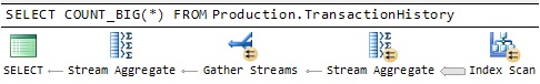
Figure 2: Parallel Counting Plan

The small yellow arrow icons identify operations that involve multiple workers. Each worker is assigned a separate part of the problem, and the partial results are then combined to give a final result. As the manual bean-counting example demonstrated, the parallel plan has the potential to complete much faster than the serial plan, because multiple workers will be actively counting rows, simultaneously.

How Parallelism Works

Imagine for a moment that SQL Server has no built-in support for parallelism. You might try to improve the performance of the original row-counting query by manually splitting the query into equally-sized pieces, and running each one concurrently on a separate connection to the server.

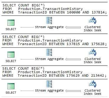
Figure 3: Manual Parallelism

Each query in Figure 3 is written to process a separate range of rows from the table, ensuring that every row from the table is processed exactly once overall. With luck, SQL Server would run each query on a separate processing unit, and you could expect to receive the three partial results in roughly a third of the time. Naturally, you would still need to perform the extra step of adding the three values together to get a correct final result.

Parallel Execution as Multiple Serial Plans

The ‘manual parallelism’ example is not that far removed from the way SQL Server actually implements its parallel query facility. Recall the parallel query plan from Figure 2, and assume that SQL Server allocates three additional workers to the query at runtime. Conceptually, we can redraw the parallel plan to show SQL Server running three serial plans concurrently (this representation is not strictly accurate, but we will correct that shortly).

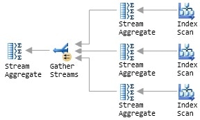
Figure 4: Multiple Serial Plans

Each additional worker is assigned to one of the three plan branches that feed into the Gather Streams operator. Notice that only the Gather Streams operator retains the little yellow parallelism icon; it is now the only operator that interacts with multiple workers. This general strategy suits SQL Server for two main reasons. Firstly, all the SQL Server code necessary to execute serial plans already exists, and has been optimized over many years and product releases. Secondly, this method scales extremely well: if more workers are available at runtime, SQL Server can easily add extra plan branches to split the work more ways.

The number of extra workers SQL Server assigns to each parallel plan region at runtime is known as the degree of parallelism (often abbreviated to DOP). SQL Server chooses the DOP just before the query starts executing, and it can change between executions without requiring a plan recompilation. The maximum DOP for each parallel region is determined by the number of logical processing units visible to SQL Server.

Parallel Scan and the Parallel Page Supplier

The problem with the conceptual plan shown in Figure 4 is that each Index Scan operator would count every row in the entire input set. Left uncorrected, the plan would produce incorrect results and probably take longer to execute than the serial version did. The manual parallelism example avoided that issue by using an explicit WHERE clause in each query to split the input rows into three distinct and equally-sized ranges.

SQL Server does not use quite the same approach, because distributing the work evenly makes the implicit assumption that each query will receive an equal share of the available processing resources, and that each data row will require the same amount of effort to process. In a simple example like counting rows in a table (on a server with no other activity) those assumptions may well hold, and the three queries might indeed return their partial results at about the same time.

In general, however, it is easy to think of examples where one or more of those hidden assumptions would not apply in the real world, due to any number of external or internal factors. For example, one of the queries might be scheduled on the same logical processor as a long-running bulk load, while the others run without contention. Alternatively, consider a query that includes a join operation, where the amount of effort required to process a particular row depends heavily on whether it matches the join condition or not. If some queries happen to receive more joining rows than others, the execution times are likely to vary widely, and overall performance will be limited by the speed of the slowest worker.

Instead of allocating a fixed number of rows to each worker, SQL Server uses a Storage Engine feature called the Parallel Page Supplier to distribute rows among the workers, on demand. You will not see the Parallel Page Supplier in a graphical query plan because it is not part of the Query Processor, but we can extend the illustration of Figure 4 to show where it would sit and what its connections would be:

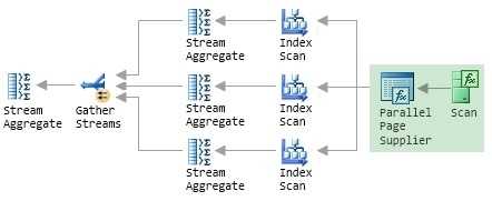
Figure 5: The Parallel Page Supplier

The crucial point is that this is a demand-based scheme; the Parallel Page Supplier responds to requests from workers, providing a batch of rows to any worker that needs more work to do. Referring back to the bean-counting analogy, the Parallel Page Supplier is represented by the scoop used to remove beans from the jar. The single, shared scoop ensures that no two people count the same beans, but there is otherwise nothing to stop the same person collecting more beans, as required. In particular, if one person is slower than the others, that person simply takes fewer scoops from the jar, and the other workers will count more beans to compensate.

In SQL Server, a slow worker makes fewer requests to the Parallel Page Supplier, and so processes fewer rows. Other workers are unaffected, and continue to process rows at their individual maximum rates. In this way, the demand-based scheme provides some measure of resilience to variations in worker throughput. Instead of being bound by the speed of the slowest worker, the performance of the demand scheme degrades gracefully as individual worker throughput declines. Nevertheless, the fact that each worker may process a significantly different number of rows, depending on runtime conditions, can cause other problems (a topic we will return to later in this series).

Note that the use of a Parallel Page Supplier does not prevent SQL Server from using existing optimizations like read-ahead scanning (prefetching data from permanent storage). In fact, it may even be slightly more efficient for the three workers to consume rows from a single, underlying physical scan, rather than from the three separate range scans that we saw in the manual parallelism example.

The Parallel Page Supplier is also not limited to use with index scans; SQL Server uses a Parallel Page Supplier whenever multiple workers cooperatively read a data structure. That data structure may be a heap, clustered table, or an index, and the operation may be either a scan or a seek operation. If the latter point surprises you, consider that an Index Seek operation is just a partial scan i.e. it seeks to find the first qualifying row and then scans to the end of the qualifying range.

Execution Contexts

We now turn to the separate server connections, used in the manual parallelism example to allow concurrent execution. It would not be efficient for SQL Server to actually create multiple new connections for each parallel query executed, but the real mechanism is similar in many ways. Instead of creating a separate connection for each serial query, SQL Server uses a lightweight construct known as an execution context.

An execution context is derived from part of the query plan, at runtime, by filling in details that were not known at the time the plan was compiled and optimized. These details include references to objects that do not exist until runtime (a temporary table created within the same batch, for example) and the runtime values of any parameters and local variables. For more details on execution contexts, see this Microsoft White Paper.

SQL Server runs a parallel plan by deriving DOP execution contexts for each parallel region of the query plan, using a separate worker to run the serial plan portion contained in each context. To help visualise the concept, Figure 6 shows the four execution contexts created for the parallel counting plan we have been working with so far. Each colour identifies the scope of an execution context, and although it is not shown explicitly, a Parallel Page Supplier is again used to coordinate the index scans.

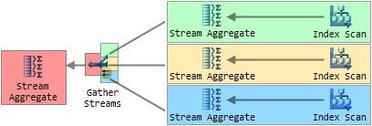
Figure 6: Parallel Plan Execution Contexts

The leftmost execution context of a parallel query plan (the one shown in red, in Figure 6) plays a special coordinating role and is executed by the worker provided by the connection that submitted the query. This ‘first’ execution context is known as execution context zero, and the associated worker is known as thread zero. We will define some of these terms more precisely in the next section, but for now assume that ‘worker’ and ‘thread’ mean roughly the same thing.

To provide a more concrete view of the abstract concepts introduced in this section, Figure 7 shows information obtained by running the parallel row-counting query, with the SQL Server Management Studio (SSMS) option, ‘Include Actual Execution Plan’, turned on.

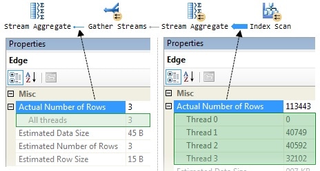
Figure 7: Parallel Plan Row Counts

The callouts show the number of rows processed by each worker (thread) at two different points in the plan. The information comes from the SSMS Properties window, which can be accessed by clicking on an operator (or connecting line) and pressing F4. Alternatively, you can right-click an operator or line and choose Properties from the pop-up menu.

Reading from the right, we see row counts for each of the three workers in the parallel part of the plan; notice that two workers processed a similar number of rows (around 40,000), but the third obtained just 32,000 rows from the Parallel Page Supplier. As discussed, the demand-based nature of the process means that the precise number of rows processed by each worker depends on timing issues and processor load (among other things) and often varies between executions, even on a lightly-loaded machine.

The left-side of the diagram shows the three partial results (one from each parallel worker, executing in its own execution context) being collected together and summed to a single result by ‘thread zero’. It is a quirk of the SSMS Properties window that ‘thread zero’ is labelled as ‘Thread 0’ in parallel parts of a graphical plan, and as ‘All threads’ in a serial region. If you look instead at the XML on which the graphical plan is based, the ‘Runtime Counters Per Thread’ element always refers to thread 0, never ‘All threads’.

Schedulers, Workers, and Tasks

This article has so far used terms like ‘thread’ and ‘worker’ somewhat interchangeably. Now seems like a good time to define some terms a little more precisely.

Schedulers

A scheduler in SQL Server represents a logical processor, which might physically be a CPU, a processor core, or perhaps one of several hardware threads running within a core (hyperthreading). The primary purpose of a scheduler is to allow SQL Server precise control over its own thread scheduling, rather than relying on the generic algorithms used by the Windows operating systems. Each scheduler ensures that only one cooperatively-executing thread is runnable (as far as the Operating System is concerned) at any given moment, which has important benefits such as reduced context-switching, and a reduced number of calls into the Windows kernel. Part three of this series covers the internals of task scheduling and execution in much more detail.

Information about schedulers is shown in the system dynamic management view (DMV), sys.dm_os_schedulers.

Workers and Threads

A SQL Server worker is an abstraction that represents either a single operating system thread or a fiber (depending on the configuration setting ‘lightweight pooling‘). Very few systems run with fiber-mode scheduling enabled, so many texts (including much of the official documentation) refer to ‘worker threads’ – emphasising the fact that, for most practical purposes, a worker is a thread. A worker (thread) is bound to a particular scheduler for its entire lifetime. Information about workers is shown in the DMV sys.dm_os_workers.

Tasks

Books Online has this to say about tasks:

A task represents a unit of work that is scheduled by SQL Server. A batch can map to one or more tasks. For example, a parallel query will be executed by multiple tasks.

To expand on that rather terse definition, a task is a piece of work performed by a SQL Server worker. A batch that contains only serial execution plans is a single task, and will be executed (from start to finish) by the single connection-provided worker. This is the case even if execution has to pause to wait for another event to complete (such as a read from disk). A single worker is assigned one task, and cannot perform any other tasks until it is fully completed.

Execution Contexts

If a task describes the work to be done, an execution context is where that work takes place. Each task runs inside a single execution context, identified by the exec_context_id column in the sys.dm_os_tasks DMV (you can also see execution contexts using the ecid column in the backward-compatibility view sys.sysprocesses).

The Exchange Operator

To recap briefly, we have seen that SQL Server executes a parallel plan by concurrently running multiple instances of a serial plan. Each serial plan is a single task, run by a dedicated worker thread inside its own execution context. The final ingredient in a parallel plan is the exchange operator, which is the ‘glue’ SQL Server uses to connect together the execution contexts of a parallel plan. More generally, a complex query plan might contain any number of serial or parallel regions, connected by exchange operators.

So far, we have seen just one form of the exchange operator, namely Gather Streams, but it can appear in graphical plans in two further forms:

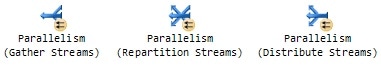
Figure 8: Exchange Logical Operations

All forms of the exchange operator are concerned with moving rows between one or more workers, distributing the individual rows among them as it goes. The different logical forms of the operator are used by SQL Server to introduce a new serial or parallel region, or to redistribute rows at the interface between two parallel regions.

The single physical exchange operator is even more flexible than its three logical forms might suggest. Not only can it split, combine, or redistribute rows among the workers connected to it, it can also:

• Use one of five different strategies to determine to which output to route an input row
• Preserve the sort order of the input rows, if required
• Much of this flexibility stems from its internal design, so we will look at that first.

Inside an Exchange

The exchange operator has two distinct sub-components:

• Producers, which connect to the workers on its input side
• Consumers, which connect to workers on its output side

Figure 9 shows a magnified view of the (multi-coloured) Gather Streams operator, from Figure 6.

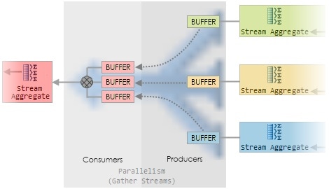
Figure 9: Inside a Gather Streams Exchange

Each producer collects rows from its input and packs them into one or more in-memory buffers. Once a buffer is full, the producer pushes it to the consumer side. Each producer and consumer runs on the same worker thread as the execution context to which it is connected (as indicated by the common colours). The consumer side of the exchange reads a row from an exchange buffer whenever it is asked for one by its parent operator (the red-shaded Stream Aggregate in this case).

One of the major benefits of this design is that the complexities normally associated with sharing data between multiple threads of execution can be handled by SQL Server inside one operator. The other, non-exchange operators in the plan are all running serially, and do not have to be concerned with such things.

The exchange operator uses buffers to minimize overheads and to implement a basic kind of flow control (to prevent fast producers getting too far ahead of a slow consumer, for example). The precise arrangement of buffers varies with the type of exchange, whether or not it is required to preserve order, and how it decides to which consumer a producer row should be routed.

Routing Rows

As noted, an exchange operator can decide to which consumer a producer should route a particular row. This decision depends on the Partitioning Type specified for the exchange, and there are five options.

Partitioning Type	Description
Hash	Most common. The consumer is chosen by evaluating a hash function on one or more column values in the current row.
Round Robin	Each new row is sent to the next consumer in a fixed sequence.
Broadcast	Each row is sent to all consumers.
Demand	The row is sent to the first consumer that asks for one. This is the only partitioning type where rows are pulled from the producer by the consumer inside the exchange operator.
Range	Each consumer is assigned a non-overlapping range of values. The range into which a particular input column falls determines which consumer gets the row.

The Demand and Range partitioning types are much less common than the first three, and are generally only seen in query plans that operate on partitioned tables. The Demand type is used in collocated partitioned joins to assign a partition id to the next worker thread. The Range partitioning type is used, for example, when creating partitioned indexes. The type of partitioning used, and any column values used in the process, is visible in the graphical query plan:

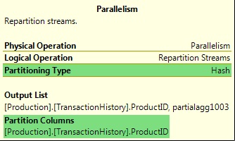
Figure 10: Exchange Partitioning Information

The more common partitioning types will be covered in detail later in the series.

Preserving Input Order

An exchange operator may optionally be configured to preserve sort order. This is useful in plans where rows entering the exchange are already sorted (following an earlier sort, or as a consequence of an ordered read from an index) in a way that is useful to a later operator. If the exchange did not preserve order, the optimizer would have to introduce an extra Sort operator after the exchange to re-establish the required ordering. Common operators that require sorted inputs include Stream Aggregate, Segment, and Merge Join. Figure 11 shows an order-preserving Repartition Streams exchange in action:

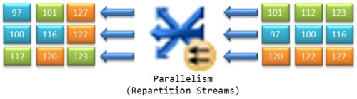
Figure 11: An Order-Preserving Repartition Streams Exchange

Rows arriving on the three inputs to the exchange are in sorted order (sorted, that is, from the point of view of the individual workers). An order-preserving exchange, known as a merging exchange, ensures that the worker(s) on its output side receive rows in the same sort order (though the distribution will usually be different, of course).

A Gather Streams exchange can also preserve sort order, if required (and Distribute Streams exchange has no other option, if you think about it). In any case, if the exchange is a merging exchange, the exchange operator has an ‘Order By‘ attribute, as shown in Figure 12:

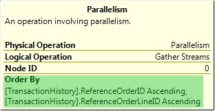
Figure 12: The ‘Order By’ Attribute of a Merging Exchange

Note that a merging exchange does not perform any sorting itself; it is limited to preserving the sort order of rows arriving on its inputs. Merging exchanges can be much less efficient than the non-order-preserving variety, and are associated with certain performance problems. This is another topic we will cover in more detail later on in the series.

Summary

This introduction to parallelism used a simple query, and a related real-world example, to explore the model used by SQL Server to allow queries to automatically benefit from the extra processing power provided by modern multi-core servers, without requiring the developer to consider any of the complexities normally associated with multi-threaded designs.

We saw that a parallel query plan may contain any number of parallel and serial regions, bounded by exchange operators. The parallel zones expand into multiple serial queries, each of which uses a single worker thread to process a task within an execution context. The exchange operators are used to route rows between workers, and are the only operators in a parallel plan that interact directly with more than one worker. Finally, we saw that SQL Server provides a Parallel Page Supplier, which allows multiple workers to cooperatively scan a table or index, while guaranteeing correct results.

The next part in this series builds on the foundations provided in this introduction, and looks at how execution contexts, worker threads, and exchange operators are applied to queries using parallel hash and merge joins. We will also look at exchange partitioning types in more detail, and examine a query optimization that is only possible in parallel plans; one which can result in a parallel query using less processor time than the equivalent serial query, while also returning results more quickly.