A function, in any programming environment, lets you encapsulate reusable logic and build software that is “composable”, i.e. built of pieces that can be reused and put together in a number of different ways to meet the needs of the users. Functions hide the steps and the complexity from other code.

However, in certain respects, SQL Server’s functions are fundamentally different from functions in other programming environments. In procedural programming, the piece of functionality that most programmers call a function should really be called a subroutine, which is more like a miniature program. These subroutines can go about changing data, introducing side effects, and generally misbehaving as much as they like.

In SQL Server, functions adhere much more closely to their mathematic definition of mapping a set of inputs to a set of outputs. SQL Server’s functions accept parameters, perform some sort of action, and return a result. They do all of this with no side effects. Nevertheless, in the same way as subroutines, SQL Server functions can hide complexity from users and turn a complex piece of code into a re-usable commodity. Functions make it possible, for example, to create very complex search conditions that would be difficult and tedious to express in inline T-SQL.

This article describes:

• The types of user-defined functions (UDFs) that SQL Server supports, both scalar (which return a single value) and table-valued (which return a table), and how to use them.
•  Some of the more interesting built-in functions
• How and why functions can get you into trouble, and cause terrible performance, if you’re not careful about how you use them.

Fun Facts about Functions

This section describes, briefly, some of the basic characteristics of the various types of SQL Server function, which we’ll explore in more detail as we progress through the later examples.

As noted in the introduction, all SQL Server functions adhere closely to the mathematic definition of a function i.e. a mapping of inputs to outputs, without have side effects. A function with inputs x and y cannot both return x + y and modify the original value of y. As a matter of fact, that function couldn’t even modify y:  it is only able to return a new value.

Where Can I Use A Function?

Anywhere!

Well, we can use a function almost anywhere that we would use a table or column. We can use a function anywhere that we can use a scalar value or a table. Functions can be used in constraints, computed columns, joins, WHERE clauses, or even in other functions. Functions are an incredibly powerful part of SQL Server.

Functions can be Scalar or Table-valued

Scalar functions return a single value. It doesn’t matter what type it is, as long as it’s only a single, value rather than a table value. You can use a scalar function “anywhere that a scalar expression of the same data type is allowed in T-SQL statements” (quote from Books Online). All data types in SQL Server are scalar data types, with the exception of TEXT, NTEXT, ROWVERSION, and IMAGE. Unless you are working with SQL Server 2000, you should be avoiding the TEXT, NTEXT, and IMAGE data types; they are deprecated and will be removed in a future version of SQL Server.

In addition to user-defined scalar functions, SQL Server provides numerous types of built-in scalar functions, some of which we’ll cover in more detail later. For example, there are several built-in date functions, such as GETDATE, string functions, such as SUBSTRING, and so on, all of which act on a single value and return a single value. There are also aggregate functions that perform a calculation on a set of values and return a single value, as well as a few ranking functions that produce one row for each input row.

Table-valued functions (TVFs) return a table instead of a single value. A table valued function can be used anywhere a table can be used – typically in the FROM clause of a query. TVFs make it possible to encapsulate complex logic in a query. For example, security permissions, calculations, and business logic can be embedded in a TVF. Careful use of TVFs makes it easy to create re-usable code frameworks in the database.

One of the important differences between scalar functions and TVFs is the way in which they can be handled internally, by the SQL Server query optimizer.

Most developers will be used to working with compilers that will “inline” trivial function calls. In other words, in any place where the function is called, the compiler will automatically incorporate the whole body of the function into the surrounding code. The alternative is that a function is treated as interpreted code, and invoking it from the main body of code requires a jump to a different code block to execute the function.

The biggest drawback of SQL Server functions is that they may not be automatically inlined. For a scalar function that operates on multiple rows, SQL Server will execute the function once for every row in the result set. This can have a huge performance impact, as will be demonstrated later in the article. Fortunately, with TVFs, SQL Server will call them only once, regardless of the number of rows in the result set and it’s often possible, with a bit of ingenuity, to rewrite scalar functions into TVFs, and so avoid the row-by-row processing that is inherent with scalar functions.

In some cases, it might be necessary to dispense with the TVF altogether, and simply “manually inline” the function logic into the main code. Of course this defeats the purpose of creating a function to encapsulate re-usable logic.

Functions can be Deterministic or Nondeterministic

A deterministic function will return the same result when it is called with the same set of input parameters. Adding two numbers together is an example of a deterministic function.

A nondeterministic function, on the other hand, may return different results every time they are called with the same set of input values. Even if the state of the data in the database is the same, the results of the function might be different. The GETDATE function, for example,  is nondeterministic. One caveat of almost all nondeterministic functions is that they are executed once per statement, not once per row. If you query 90,000 rows of data and use the RAND function to attempt to produce a random value for each row you will be disappointed; SQL Server will only generate a single random number for the entire statement. The only exception to this rule is NEWID, which will generate a new GUID for every row in the statement.

When we create a function, SQL Server will analyze the code we’ve created and evaluate whether  the function is deterministic. If our function makes calls to  any nondeterministic functions, it will, itself, be marked as nondeterministic. SQL Server relies on the author of a SQL CLR function to declare the function as deterministic using an attribute.

Deterministic functions can be used in indexed views and computed columns whereas nondeterministic functions cannot.

Keeping things safe: functions can be schema-bound

Functions, just like views, can be schema bound. Attempts to alter objects that are referenced by a schema bound function will fail. What does this buy us, though? Well, just as when schema binding a view, schema binding a function makes it more difficult to make changes to the underlying data structures that would break our functions. To create a schema-bound function we simply specify schema binding as an option during function creation, as shown in Listing 1.

Listing 1: Creating a Schema Bound Function

Behavior around NULL

We can bind a function to our database schema, thereby preventing database changes  breaking our function, but what do we do when our function receives NULL input values? By default, SQL Server will go ahead and run the code in the function and evaluate all of the parameters passed in, even if one of those parameters is a NULL value, and so the output of the function is NULL.

This is a waste of processor cycles and we need to avoid this unnecessary work. We could check every parameter that is passed into a function, but that is a lot of code to maintain. If you’re thinking, “there has to be a better way” then you’re absolutely right. When we create the function we can use the RETURNS NULL ON NULL INPUT option, which will cause SQL Server to immediately return NULL if any parameters in the function are NULL-valued. Users of SQL Server 2000 and earlier are out of luck, though, as this feature was introduced in SQL Server 2005.

Scalar User-defined Functions

It’s time to take a look at some interesting uses for scalar UDFs, and along the way elucidate the rules that govern how we create and call them.

Calling Scalar UDFs

There are a few rules that must be followed when creating a function:

• The body of the function must be enclosed in a BEGIN/END block.
• Statements with side effects (insert/update/delete) and temporary tables may not be used. You can, however, use table variables. Table variables are allowed in UDFs because they are created as variables, not through DDL. DDL is viewed as producing a side effect and is not allowed.
• TRY/CATCH statements are not allowed since CATCH can have the side effect of masking the error state of a given function.

Let’s dive straight in and take a look at Listing 2, which shows the code to create, in the AdventureWorks2008 database, a scalar UDF called ProductCostDifference, which will compute the cost difference for a single product, over a time range.

Listing 2: Creating a scalar function

Likewise, when we call a UDF, we must follow a few rules:

•  quality the function name (e.g. Production.ProductCostDifference) when using a function in a query.
• Optional parameters cannot be omitted, but we can use the DEFAULT keyword to supply the default value.

Listing 3 shows a simple call to our ProductCostDifference function.

Listing 3: Executing a user-defined function

Scalar UDFs are a fairly straightforward feature but there are some drawbacks to them, the biggest one being that, as discussed earlier, SQL Server has no optimization whereby it can compile this function as inline code. Therefore, it will simply call it once for every row to be returned in the result set. Another drawback of scalar UDFs is that we won’t see the true cost of the function when we’re looking at execution plans. This makes it difficult to gauge just how much a UDF is hurting query performance.

Scalar functions in the SELECT Clause

Listing 4 demonstrates calling our function in the SELECT statement of two simple queries, the only difference being that in the second query we filter out NULL results from our scalar function.

Listing 4: Running a query with a scalar function

Unfortunately, SQL Server is not terribly intelligent in the way that it works with scalar functions. In the first query, our ProductCostDifference function will be executed once for each of the 504 rows in the Production.Product table. This leads to an increase in disk access, CPU utilization, and memory utilization. The execution plan for this query is shown in Figure 1.

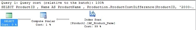
Figure 1: Execution Plan for Query 1 in Listing 4

We can see that all data is read from disk in the Index Scan operator before being sent to the Compute Scalar operator, where our function is applied to the data. If we open up the Properties page for the Compute Scalar node (pressing F4 will do this if you haven’t changed the default SQL Server Management Studio settings) and examine the Define Values property list. If this references the function name (rather than the column name), as it will in this case, then the function is being called once per row.

The situation is even worse for the second query in Listing 4 in that the function needs to be evaluated twice: once for every 504 rows in the Production.Product table and once again for the 157 rows that produce a non-NULL result from our scalar function. The execution plan for this query is shown in Figure 2.

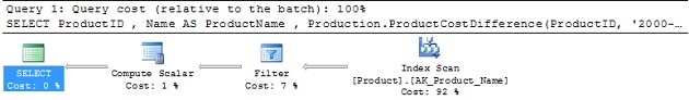
Figure 2: Execution Plan for Query 2 in Listing 4

Again, we can establish whether or not a function is being executed once per row by examining the details of this plan; in this case, the properties of either the Compute Scalar or the Filter node. The Predicate property of the Filter node shows that that the filter operation is filtering on:

[AdventureWorksCS].[Production].[ProductCostVariance]([AdventureWorksCS].[Production].[Product].[ProductID],'2000-01-01 00:00:00.000',getdate()) IS NOT NULL.

In other words, SQL Server is evaluating the function once for every row in the product table. No function ‘inlining’ has been performed; we would be able to see the ‘inlined’ source code if it had been.

This may seem like a trivial point to labor over, but it can have far reaching performance implications. Imagine that you have a plot of land. On one side of your plot of land is a box of nails. How long would it take you to do anything if you only used one nail at a time and kept returning to the box of nails every time you needed to use another one? This sort of thing might not be bad for small tasks like hanging a picture on the wall, but it would become incredibly time consuming if you were trying to build an addition for your house. The same thing is happening within your T-SQL. During query evaluation, SQL Server must evaluate the output of the scalar function once per row. This could require additional disk access and potentially slow down the query.

Scalar functions, when used appropriately, can be incredibly effective. Just be careful to evaluate their use on datasets similar to the ones you will see in production before you make the decision to use them; they have some characteristics that may cause undesirable side effects. If your scalar UDF needs to work on many rows, one solution is to rewrite it as a table-valued function, as will be demonstrated a little later.

Scalar functions in the WHERE Clause

Using a scalar function in the WHERE clause can also have disastrous effects on performance. Although the symptoms are the same (row-by-row execution), the cause is different. Consider the call to the built-in scalar function, DATEADD, in Listing 5.

Listing 5: Poor use of a function in the WHERE clause

This code will result in a full scan of the Sales.SalesOrderHeader table because SQL Server can’t use any index on the OrderDate column. Instead, SQL Server has to scan every row in the table and apply the function to each row. A better, more efficient way to write this particular query would be to move the function, as shown in Listing 6.

Listing 6: Better use of a function in the WHERE clause

Optimizing the use of a function in the WHERE clause isn’t always that easy, but in many occasions this problem can be alleviated through the use of careful design, a computed column, or a view.

Constraints and Scalar Functions

Functions can be used for more than just simplifying math; they are also a useful means by which to encapsulate and enforce rules within the data.

Default Values

Functions can be used to supply the default value for a column in a table. There is one requirement: no column from the table can be used as an input parameter to the default constraint.

In Listing 7, we create two tables, Bins and Products, and a user defined function, FirstUnusedProductBin, which will find the first unused bin with the fewest products. We then use the output of the FirstUnusedProductBin function as a default value for the BinID in the Products table. Creating this default value makes it possible to have a default storage location for products, which can be overridden by application code, if necessary.

Listing 7: Creating a table with a UDF default

Our UDF will only work for single row INSERTs. We’ll explore what happens with a set-based INSERT after we look at the function working correctly with single row INSERTs.

Listing 8: Modifying data in the Products table

When we insert data into the Products table in the first statement it’s very easy to see that every bin is filled. If we remove one product and add a different product, the empty bin will be re-used.

Although this example demonstrates nicely the way in which we can use functions to set default values, the implementation of this function is naïve; once all bins are full it will circle around and begin adding products to the least full bin. An ideal function would use a bin-packing algorithm. If you need to use a bin-packing algorithm in T-SQL, I recommend looking at Chapter 4: Set-based iteration in SQL Server MVP Deep Dives (Kornelis 2009).

What happens if we try to INSERT more than one row at a time?

Listing 9: Inserting many rows at once

Every row is inserted with the same default value. The FirstUnusedProductBin function is only called once for the entire transaction. A better way to enforce a default value that works for both single-row INSERTs and multi-row INSERTs is to use an INSTEAD OF trigger to bypass the set-based INSERT. In effect, we have to force SQL Server to use row-by-row behavior in order to insert a new value in each row.

Listing 10: A Multi-row solution

To provide a constantly changing default value for each row we’ve removed the default constraint and replaced it with an INSTEAD OF trigger for the INSERT. Unfortunately, this trigger adds significant overhead, but it does demonstrate the difficulty of using functions to enforce complex default constraints.

Enforcing Constraints with Functions

Scalar UDFs are often very useful for data validation and restriction. Many constraints enforce simple, inline evaluations, such as the “number of federal income tax deductions must be less than ten”). For example, the CHECK constraint in Listing 11 enforces the rule that no employee’s yearly bonus is more than 25% of their salary (one could argue that this sort of salary logic belongs in the application not database, but that debate is not really relevant to our goal here).

Listing 11: A simple CHECK constraint

Say, though that we have second rule for this data says that “no employee may have a salary that is 10 times greater than the salary of the lowest paid employee”. This is a bit trickier because if we try to add a subquery to the CHECK constraint, we receive an error that “Subqueries are not allowed in this context. Only scalar expressions are allowed.” SQL server is, wisely, preventing us from comparing the output of a query with a single value. Since we cannot put this comparison inline, we’ll have to create a scalar UDF and use the function to compare the data.

Listing 12: Creating a constraint with a function

Functions in constraints are not limited to the current table; they can reference any table in the database to enforce data constraints. In the following example we will create two tables – Employees and PayGrades – and implement a CHECK constraint that prevents an employee from having the same or higher pay grade as their manager.

Listing 13: A constraint using functions that access other tables

Having now created our tables and a function to validate the business rule, we can set about testing that our rules actually work.

Listing 14: Verifying our constraints by creating data

The first two inserted rows create the head of the company at the top pay grade and then we create an immediate subordinate. The third INSERT fails because we’re attempting to create an employee at the same pay grade as their manager. When we try to insert a row that violates the check constraint, an error is returned to the client. We could parse this error message and return a meaningful message to the client instead of this:

Table-valued Functions

Table-valued Functions (TVFs) differ from scalar functions in that TVFs return an entire table whereas scalar functions only return a single value. This makes them ideal for encapsulating more complex logic or functionality for easy re-use. TVFs have the additional advantage of being executed once to return a large number of rows (as opposed to scalar functions which must be executed many times to return many values).

The body of a TVF can either contain just a single statement or multiple statements, but the two cases are handled very differently by the optimizer. If the function body contains just a single statement (often referred to as an “inline TVF”), then the optimizer treats it in a similar fashion to a view in that it will “decompose” it and simply reference the underlying objects (there will be no reference to the function in the resulting execution plan).

However, by contrast, multi-statement TVFs present an optimization problem for SQL Server; it doesn’t know what to do with them. It treats them rather like a table for which it has no available statistics – the optimizer assumes that it the TVF will always return one row. As a result, even a very simple multi-statement TVF can cause severe performance problems.

Avoiding Row-by-Row Behavior with TVFs

One of the problems with scalar functions is that they are executed once for every row in the result set. While this is not a problem for small result sets, it becomes a problem when our queries return a large number of rows. We can use TVFs to solve this problem.

We’ll start with a relatively simple case of converting a single-statement scalar function into a single-statement TVF. We’ll then move on to the slightly more complex case of converting our previous ProductCostDifference scalar function (Listing 2), which contains multiple statements. As we discussed earlier, this function can only operate on a single row at a time. If we wanted to execute that function over several million rows, we would see a considerable spike in disk I/O and a decrease in performance.

Single-statement Scalar to Single-statement TVF

Let’s take a look at a new example, looking at order data from the AdventureWorks database. We are specifically interested in the average weight of orders so we can determine if we need to look into different shipping options.

Listing 15 creates two functions; the first is a scalar function and will compute the order weight for any single order. This is ideal for queries showing the details of a single order or a few orders, but when it comes to working with a large number of orders this could cause an incredible amount of disk I/O. The second function is a single-statement table-valued function that performs the exact same calculation, but does so over an entire table instead of for a single row.

Listing 15: Two functions for Finding Order Weight

Listing 16 shows the queries for calling each of these functions.

Listing 16: Using the OrderWeight Functions

Notice the different ways in which the two functions are invoked. We use our single-statement TVF the same way that we would use a table. This makes it very easy to use TVFs in our queries; we only need to join to them and their results will be incorporated into our existing query.

When you hit the Execute button for those queries, it should be immediately clear that one of them, at least, is pretty slow. However, by examining the execution plans alone, as shown in Figure 6, it’s hard to tell which one is the culprit. In fact, in terms of relative plan cost, you may even conclude that the first plan is less expensive.

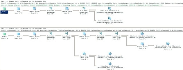
Figure 3: Execution plans for calling the scar function and the TVF

Unfortunately, the top execution plan (for the scalar function), hides any immediately-obvious evidence of the Sales.OrderWeight function reading row-by-row through the Sales.SalesOrderDetail table. Our evidence for that comes, again, from the Compute Scalar operator, where we see direct reference to our Sales.OrderWeight function, indicating that it is being called once per row.

In the second execution plan, for the TVF, we see the index scan against the Sales.SalesOrderDetail table. Our TVF is called just once to return the required rows, and has effectively been “inlined”; the plan references only the underlying objects with no reference to the function itself.

Using SET STATISTICS TIME ON revealed that (one my machine) the first query executes in 28 seconds while the second query executes in 0.6 seconds. Clearly the second query is faster than the first.

Later in the article, we’ll take this a step further and show how to dispense with the TVF altogether and manually inline the logic of this TVF; a strategy that’s sometimes advantageous from a performance perspective.

Multi-statement Scalar to Multi-statement TVF

Let’s now look at the more complex case of converting our multi-statement ProductCostDifference scalar function into a TVF. We’re going to start with a straight conversion to a multi-statement TVF.

As noted, a multi-statement TVF is one that contains more than one statement in the function body. Listing 17 shows a nearly-direct translation of the original scalar function, in Listing 2, into a multi-statement table-valued function.

Listing 17: A multi-statement TVF

This TVF, Instead of retrieving a single row from the database and calculating the price difference, pulls back all rows from the database and calculates the price difference for all rows at once.

Listing 18: Using the TVF

The downside of this multi-statement TVF is that SQL Server makes the assumption that only one row will be returned from the TVF, as we can see from the execution plan in Figure 4. With the data volumes we see in AdventureWorks, this doesn’t pose many problems. On a larger production database, though, this would be especially problematic.

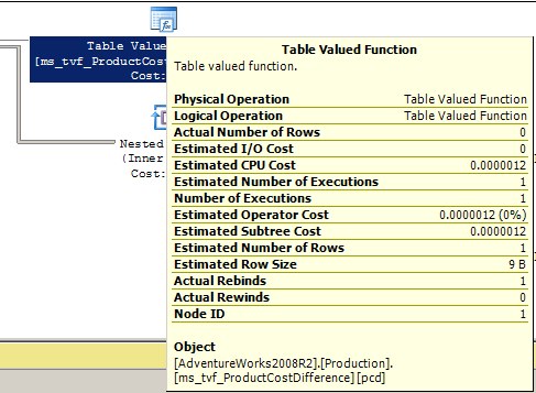
Figure 4: Only one row

Multi-statement Scalar to Single-statement TVF

Let’s now rewrite our original ProductCostDifference scalar function a second time, this time turning it into a single-statement (or “inline”) TVF, as shown in Listing 19.

Listing 19: Moving to a single-statement table-valued function

In addition to switching to a table valued function, we also re-wrote the code to read the table fewer times (two times, in this case; once for each use of the CTE in Listing 19) by using two different ROW_NUMBERs. Use of a common table expression also makes it easier and faster to get the oldest and newest row at the same time.

While this initially seems like a lot of complexity to get to our original goal, it all has a purpose. By re-writing the TVF to use a common table expression, we can avoid the performance problem of a multi-statement TVF.

Listing 20: Two uses of the single-statement TVF

The execution plan for the first query in Listing 20 is shown in Figure 5.

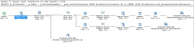
Figure 5: Execution Plan for Query 1 in Listing 20

We can see that the execution plan of the body of Production.tvf_ProductCostDifference has been “inlined”. If the query had not been inlined, we would have just seen a single operator for executing the table valued function. Note that there are two scans on ProductCostHistory, because we call the CTE twice in the function, producing two reads of the underlying query).

Again, we can confirm that this TVF is not executed once per row by examining, for example, the Compute Scalar operator, which contains no reference to our function, as well as the the Hash Match operator. If SQL Server had not inlined the function, we might have seen a nested loop join to the TVF operator.Looking at the properties of the Hash Match node, in Figure 6, we can see that SQL Server not only expects to perform the join to the body of the TVF just once, but it does perform that join only once. SQL Server has successfully inlined the TVF and it is called once for the entire result set, not once for every row.

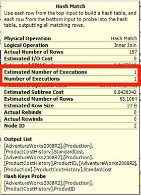
Figure 6: Properties of the Hash Match node

At this point, we’ve removed the problem we had with scalar functions, where they were executed row-by-row. We’ve also avoided the problems inherent with multi-statement TVFs. However, we still may encounter performance problems with these “inline” TVFs. The reason for this is that the TVF may be evaluated in full before being joined to our query. This means that we may see several hundred rows returned from the TVF when our query only returns a few rows. In Listing 20, we have one query that returns 157 rows and a second query that returns only a single row. However, turning on STATISTICS IO reveals that both queries perform the same amount of physical and logical IO, showing that we’re doing the same amount of work whether we return 157 rows or 1 row. In both cases, we perform two scans of ProductCostHistory at a cost of 10 logical reads.

When you are building your TVFs and the queries that use them, it’s important to remember that the join path may not always be what you expect. You may come to a point when you have been optimizing your queries and the performance bottleneck comes down to a single table-valued function returning a lot of data that is subsequently filtered down to a few rows.  What should you do then?

Rewriting TVFs with CROSS APPLY

In cases where you have a substantial amount of data that you need to restrict through joins and where conditions, it’s usually better from a performance perspective to dispense with the TVF altogether and simply “manually inline” the function logic; in other words, put the body of our T-SQL code inline with the calling code.

Inlining a TVF is as simple as pasting the body of the function into our query. This can have several benefits. Firstly, it makes it much easier to determine if our changes are improving performance. One of the problems of using functions is that multi-statement TVFs do not report their actual disk I/O to STATISTICS IO, but they do when you use the SQL Server Profiler. Single statement TVFs and inlined code will correctly report the disk I/O because it’s just another part of the query.

Inlining TVF code also makes it easier to create one-off changes for a single query; rather than create a new function, we can just change the code. When I start inlining code in production I add a comment in the stored procedure that pointed back to the original function. This makes it easier to incorporate any improvements that I may find in the future. Finally, by moving our function to inline code it’s much more likely that SQL Server will make effective join and table scanning choices and only retrieve the rows that are needed. As discussed, with TVFs, SQL Server might execute the query in our function first and return those rows to the outer query before applying any filtering. If SQL Server returns 200,000 rows and only needs 100, that’s a considerable waste of processing time and disk I/O. However, if SQL Server can immediately determine the number of rows that will be needed and which rows will be needed, it will make much more effective querying choices, including which indexes to use, the type of join to consider, and the whether or not to perform a parallel operation.

Bear in mind, however, that SQL Server is in general, very efficient at inlining single-statement TVFs. Listing 21 shows how to manually inline our Sales.tvf_OrderWeight TVF (from Listing 15), by using CROSS APPLY. The CROSS APPLY operator effectively tells SQL Server to invoke a table-valued function for each row returned by an outer query.

Listing 21: Using CROSS APPLY to inline the OrderWeight TVF

However, we’ll see no difference in the execution plan compared to the one we saw from calling the TVF (Figure 3). One of the benefits of using single statement TVFs is that SQL Server is frequently able to optimize the queries and inline the TVF for us. By knowing how to write optimal TVFs we can build reusable code and take advantage of SQL Server’s ability to automatically inline well-constructed TVFs.

We can also manually inline the logic of our multi-statemnt TVFs. Listing 22 shows how to do this for our tvf_ProductCostDifference function. However, again, we don’t get additional benefit in this particular case. It turns out that attempting to inline the common table expression has similar I/O implications to calling the function. Regardless of whether we leave the TVF as-is or inline the function logic using just the CTE, SQL Server will have to enter the CTE and evaluate the CTE query twice, once for each join to the CTE, and we’ll see the same amount of physical I/O in each case.

Listing 22: Re-writing a TVF with an inline function body’

If you run Listing 22, you’ll find that the execution plan for the manually-inlined code is very similar (but not identical) to the plan for calling the TVF (Figure 5) and performs similar I/O.

Best Practices for TVFs

Table-valued functions are best used when you will be performing operations on a large number of rows at once. Typically this will be something that could be accomplished through a complex subquery or functionality that you will re-use multiple times in your database. TVFs should be used when you can always work with the same set of parameters – dynamic SQL is not allowed within functions in SQL Server.

It’s best to use TVFs when you only have a small dataset that could be used in the TVF. Once you start getting into larger numbers of rows, TVFs can become very slow since all the results of the TVF query are evaluated before being filtered by the outer query. When this starts to happen it is best to inline the code. If inlining the TVF code doesn’t work, you can even look into re-writing the query slightly to use a JOIN instead of a CROSS APPLY. This might complicate the query, but it can lead to dramatic performance improvements.

A few useful Built-in Functions

To finish off this article, we’ll briefly review some of the built-in scalar functions that I’ve frequently found useful.

COALESCE

COALESCE takes an unlimited list of arguments and returns the first non-NULL expression. One of the advantages of COALESCE is that it can be used to replace lengthy CASE statements.

Listing 23: A CASE statement

The code in Listing 23 can be simplified by using COALESCE.

Listing 24: COALESCE

DATEADD and DATEDIFF

The best way to modify date and time values is by using the DATEADD and DATEDIFF functions. The DATEADD function can be used to add or subtract an interval to part of a date.

Listing 25: Modifying dates

The DATEDIFF function can be used to calculate the difference between to dates. DATEDIFF is similar to DATEADD – DATEDIFF gets the difference between two dates using the given time interval (year, months, seconds, and so on).

Listing 26: Finding the difference between two points in time

One practical use of the DATEDIFF function is to find the beginning of the current day or month.

Listing 27: Beginning of the day or month

This approach to getting the beginning of the day computes the number of days since the dawn of SQL Server time (January 1, 1900). We then add that number of days to the dawn of SQL Server time and we now have to beginning of the current hour, day, month, or even year.

SIGN

SIGN returns +1, 0, or -1 based on the expression supplied.

Listing 28: Using SIGN

STUFF

STUFF is a powerful built-in function. It inserts one string into another. In addition, it also removes a specific number of characters from one string and adds the second string in place of the removed characters. That isn’t a very clear explanation, so let’s take a look at an example.

Listing 29: Using STUFF

The STUFF function can be combined with several XML functions to create a comma-separated list of values from a table.

Listing 30: Creating a comma-separated list with STUFF

Summary

User-defined functions give us the ability to create reusable chunks of code that simplify the code we write. UDFs can be embedded in queries as single, scalar values or as table valued functions. Effective use of UDFs can increase the readability of your code, enhance functionality, and increase maintainability.