In this blog, we’re going to walk you through how to solve the issues posed by that concern. At the end of the article, we’ll also walk you through some DDL operations to load test data.

SELECT Queries in MySQL

In my introduction blog, I noted: Queries are processes composed of tasks – their performance depends directly on the performance of those tasks.

To address problems posed by SELECT queries, the first thing we need to understand is what happens when a SELECT queries are executed. Here’s what MySQL does in the background when we execute a SELECT query:

1. Our SQL client sends the query to the server to be executed.
2. A specific query execution plan is followed.
3. The result is returned.

Understanding these steps is no less vital than diving deeper into the query execution plan, and the output provided by an EXPLAIN statement execution – a query execution plan will provide us information in regards to what time MySQL takes to go through each step necessary to complete a query. The EXPLAIN statement will provide us more details in how MySQL executes the query itself.

For the purposes of this blog, we’re going to use the following table with three columns (it’s not necessary to specify the storage engine – MySQL will create the table based on the InnoDB storage engine by default if it’s not specified. In this specific scenario, the indexing part is not necessary, but if it’s specified, MySQL will create an index named “email” (indexes can have any names) on a column named “email.”) Also note the sizes of the email and username columns – in this case, emails shouldn’t be longer than 35 characters in length, and usernames shouldn’t be longer than 20.

It’s also worth noting that for the columns with the type of an integer the length of the column is deprecated starting from MySQL 8. So you might as well want to consider leaving the columns with an integer type intact without specifying a length attribute:

To insert data into the table, use INSERT or LOAD DATA INFILE – INSERT is an excellent choice if you’re dealing with smaller data sets (less than 100 million rows), while LOAD DATA INFILE can be very useful to work with big data sets. For INSERT, the syntax looks like so:

For LOAD DATA INFILE, the syntax looks like this – the FIELDS TERMINATED BY. Part of the query can be used to specify the character that terminates fields from one another (one can also specify what columns to load the data into by specifying them at the end of the query if we wish):

The Query Execution Plan

To dive deeper into the query execution plan, we can use the MySQL query profiler or dig into the richer performance schema by following the steps outlined in the MySQL documentation. For many, though, using the query schema is more difficult than going through the simpler query, so I will use the profiler:

1. Select a database, then issue a SET profiling = 1 query to enable profiling.
2. Run your query, then issue a SHOW PROFILES query to investigate all of the profiles of all queries.
3. Select the ID of the query you just ran (identify the query from the list provided by the profiler), then execute a SHOW PROFILE FOR QUERY [id] query.

Note: Query profiling with SET profiling = 1 has been deprecated since MySQL 5.6.7 and people are advised to follow the performance schema instead – the documentation will walk you through all of the necessary steps, just note that getting started with it is a little more complex than using the optimizer.

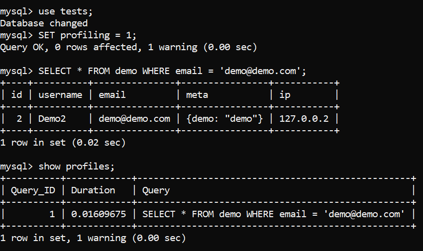
Image 1 – Profiling a Query. Initializing

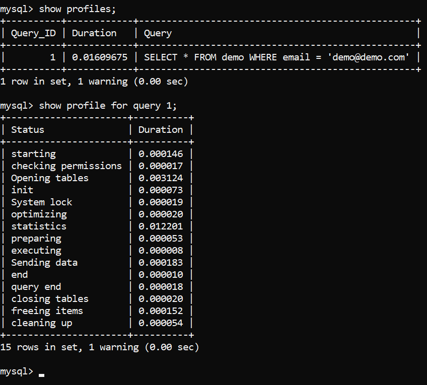
Image 2 – Profiling a Query. Results

The query execution plan is displayed above. Now we need to properly understand what’s it all about, We will start from the top and move toward the bottom (for newer versions of MySQL, the results will look a little different – there may be more items such as “Executing hook on transaction” and “waiting for handler commit”, but the core premise is the same):

1. Starting – The process of initializing the query.
2. Checking permissions – Refers to the process of MySQL checking whether the user has sufficient permissions to run the query. If permissions are not present or they are not sufficient, the process terminates here.
3. Opening tables – The process of MySQL opening all tables for operations. Once the tables are opened or if the tables are already open, MySQL proceeds to step #4.
4. Init – MySQL performs initialization processes – for example, the InnoDB log and the binary log are being flushed.
5. System lock – Once MySQL reaches this phase, it’s waiting for a system lock on the table to be released if it’s in place. In this phase, the query is making use of a function called mysql_lock_tables() and is waiting for its completion – more information can be found in the documentation, in the “System lock” paragraph.
6. Optimizing – Internal processes performed by MySQL to determine how to execute the query in the quickest way. Think of math equations – if you multiply 2 by 0, you can realize the answer is 0 in a couple of ways: by solving the equation, or by realizing that multiplying anything by 0 yields 0. That’s what MySQL does here.
7. Statistics – Calculating statistics-related data to further develop the query execution plan.
8. Preparing is pretty much self-explanatory: MySQL is preparing to run the query.
9. Executing – Once the server reaches the execution phase, the query is being executed to start producing rows for output.
10. Sending data – MySQL is doing internal work to execute the query and return the results of that query.
11. End – The end of the query before the cleanup process.
12. Query end – refers to the end of query processing.
13. Closing tables – The tables that were opened and impacted by the query are being closed.
14. Freeing items – Means that MySQL is freeing items from the thread used to execute a query.
15. Cleaning up – Finally, this stage refers to the cleaning up of items in the memory and resetting certain necessary internal variables.

For those who use the profiler, the results will be a little different, but the result will be pretty much the same. To employ the profiler, employ the following:

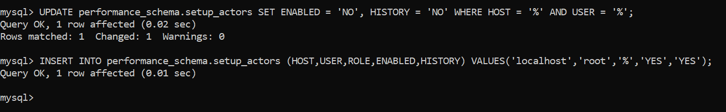
1. Tell MySQL to enable monitoring for the user that runs the query by running two queries – the first one will ensure that monitoring is off for everyone, and the second one will enable monitoring for your specific account (replace “root” with your account name):

UPDATE performance_schema.setup_actors SET ENABLED = 'NO', HISTORY = 'NO' WHERE HOST = '%' AND USER = '%';
INSERT INTO performance_schema.setup_actors (HOST,USER,ROLE,ENABLED,HISTORY) VALUES('localhost','root','%','YES','YES');

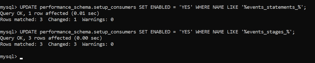
2. Enable two things – logs for statements and statement stages by running these queries:

UPDATE performance_schema.setup_consumers SET ENABLED = 'YES' WHERE NAME LIKE '%events_statements_%';

UPDATE performance_schema.setup_consumers SET ENABLED = 'YES' WHERE NAME LIKE '%events_stages_%';

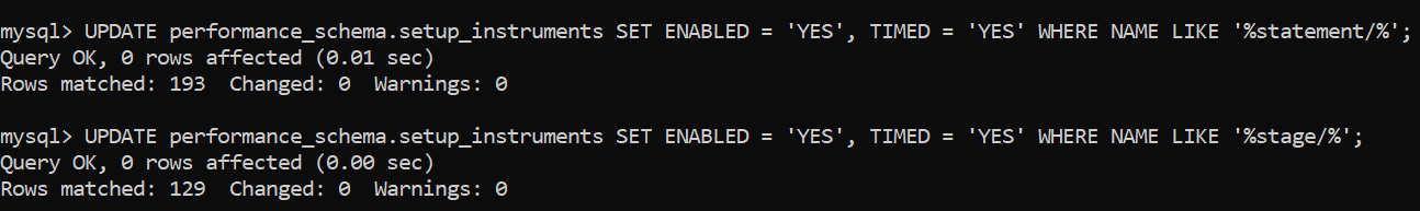
3. Update the setup_instruments table with these queries (there are no matches for me because the values are already updated):
   UPDATE performance_schema.setup_instruments SET ENABLED = 'YES', TIMED = 'YES' WHERE NAME LIKE '%statement/%';
UPDATE performance_schema.setup_instruments SET ENABLED = 'YES', TIMED = 'YES' WHERE NAME LIKE '%stage/%';

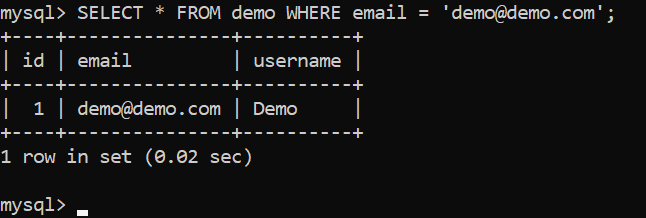
4. Finally, you can execute your query:
   SELECT * FROM demo WHERE email = 'demo@demo.com';

   
5. Now identify the query by querying the query history – run this query (replace YOUR QUERY HERE with your actual query):
   SELECT EVENT_ID, TRUNCATE(TIMER_WAIT/1000000000000,6) as Duration, SQL_TEXT FROM performance_schema.events_statements_history_long WHERE SQL_TEXT like '%YOUR QUERY HERE%';
6. Then to see the query duration and stage information, query the query history table like so (replace Query_ID with the actual query ID):
   SELECT event_name AS Stage,
TRUNCATE(TIMER_WAIT/1000000000000,6) AS Duration
FROM performance_schema.events_stages_history_long
WHERE NESTING_EVENT_ID = QUERY_ID;

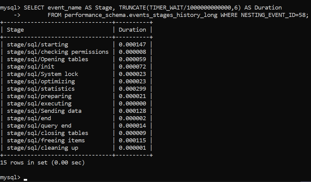
As you can see, the results don’t differ very much, and once we are aware of what the tasks in the query execution plan mean in the context of MySQL, we can start optimizing them.

Optimizing Tasks – the EXPLAIN Query

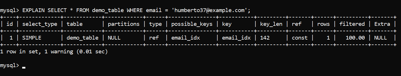
To optimize the tasks that comprise a SELECT query and make the query faster as a result, we need to take a look at the output of an EXPLAIN query that explains what the query is making use of internally. Profiling will tell us how long each query phase takes while explaining queries will tell us how the query is actually executing. Issue a SELECT query like you normally would, just add EXPLAIN at the start. We will use an example query specified below:

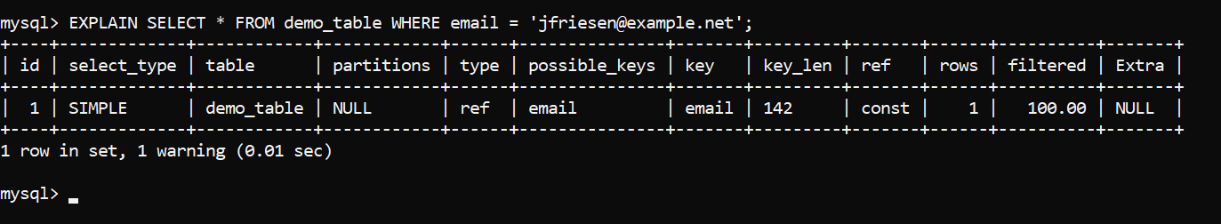
The output of the EXPLAIN query will tell us a number of things:

• The type column depicts how the row was accessed (for more information on the various methods of query access, refer to the docs. SIMPLE in this case refers to the fact it doesn’t use a UNION or subquery)
• The table column will tell you what table the SELECT query is running on. For some, it may be self-explanatory, but if you run a lot of SELECT statements, such a feature is useful. The documentation has more information on its functionality.
• The partitions column will tell you whether partitions are used, and if so, what their names are.
• The possible_keys column describes the indexes MySQL could have chosen. The key column provides us with the chosen index, and the key_len column depicts the length of the index on that column. Do note that the key length is the index length – not the length of data (it will not be the same as defined in the data type.) In this case, the length of the index (the key length) is also calculated internally by MySQL, thus the value of “142.” More information on possible indexes can be found here, and indexes are covered here.
• The ref column tells us what columns were working with the index in question to select data. In other words, MySQL is searching for columns that are working with the index as described in the docs.
• The rows column depicts the number of rows in the table. Bear in mind that for InnoDB, this number is likely to be an estimate rather than the actual value because InnoDB doesn’t store the row count internally as MyISAM does – more information can be found in the documentation over here.
• The filtered column shows an estimate of how many rows are going to be filtered out (i.e. not included in the result set.) The percentage given in this column is only an estimate, so don’t be surprised if you see “100.00” like in the example above. More information on this value can be found here.
• There are also other possible values, like the select_type value: the select_type value outlines the type of SELECT that was used (if the SELECT used a UNION clause, etc.)

To better understand the results of profiling and the EXPLAIN query, keep in mind the following:

1. A SELECT query will be blazing fast if it scans through as few rows as possible. Hence, we should avoid selecting all columns for a result set – only selecting necessary columns will be enough.
2. The main thing that optimizes the performance of a SELECT query is indexes (also called keys.) Look closely at the output of the EXPLAIN query – the “possible_keys” column depicts the indexes that MySQL can use, and the “key” column depicts what index was actually chosen. Indexes make SELECT queries faster because when an index is used, MySQL doesn’t read through all data to find a column value (refer to point #1.)

   Indexes have multiple types (we will tell you what they are in a second), and indexes do really deserve a book in and of themselves, so for those who are interested in how they work on a deeper level, we suggest you read about everything surrounding them in the documentation of MySQL or read Relational Database Index Design and the Optimizers by Tapio Lahdenmaki and Mike Leach.

3. SELECT query performance can be significantly improved by using partitions too. Partitions essentially split tables into multiple different tables internally. Since those tables are still treated as one table by the storage engine layer, it’s usually used to store only data that begins with, say, only a specific character or number. A query then uses the data in the partition and makes the SELECT query faster because we adhere to the point #1.

Indexes and partitions are two things that are used the most frequently when optimizing SELECT queries – each of them has multiple types unique to themselves.

Both indexes and partitions help optimize SELECT query performance because indexes let MySQL find rows with specific column values in a quick fashion, and partitions act as tables within tables – MySQL can turn to them when a search query begins with a specific character to only read through the table of rows beginning with that character. As a result, SELECT statements are faster in both cases.

Types of Indexes

Indexes can be split into a couple of types – we can have B-Tree, R-Tree (spatial), and hash indexes. All indexes except spatial indexes and hash indexes are B-Tree indexes whereas spatial indexes are R-Tree indexes. There are also hash indexes, which are only supported by the MEMORY storage engine:

1. B-Tree: such indexes are the most frequently used type of index and it’s easy to understand why – they improve the performance of queries that search for exact matches of data, use the less than (“<”), more than (“>”) operators, or operators with an equal sign (“>=”, etc.): they are also used when wildcards are in use (not in all cases, though – we’ll get into that in a moment.)
   B-Tree indexes are sorted tree structures that are suited for databases that deal with a lot of data due to its ability to traverse a tree from top to bottom in a recursive fashion. Due to the fact that B-Tree indexes are sorted, exact searches (searches with the “=” operator) are made blazing fast.
2. R-Tree, or spatial, indexes are used when DBAs are running operations on geographical data.
3. Hash indexes are used for exact matches of data (i.e. only queries that use either the “=” or the “<=>” operators.) but only within the MEMORY storage engine

Index Properties

Indexes also have multiple properties that need to be discussed:

1. Covering indexes cover all of the columns required for a query to execute and when they are in use, MySQL can read them instead of reading the data. Since reading the index is significantly faster than reading the data, queries also finish quickly.
   Such indexes are pretty self-explanatory: include all of the columns used by the query in the index, and you have a covering index. Woohoo!
2. Composite indexes are sometimes confused with covering indexes, but they’re not the same; composite indexes cover multiple columns, but these columns may not necessarily be the columns that a specific query might be using.
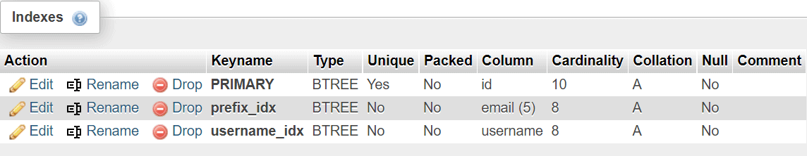
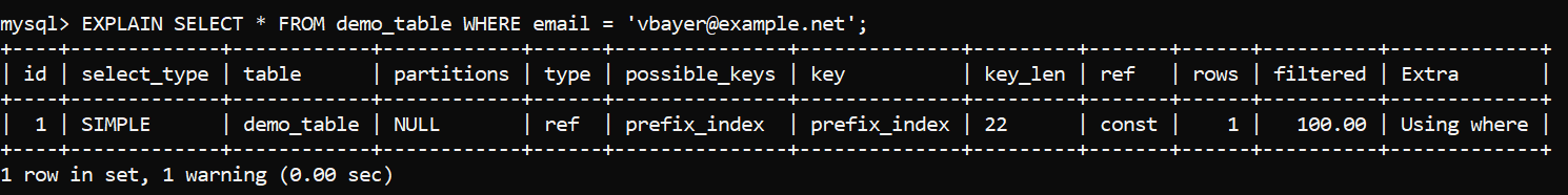
3. Prefix indexes index a prefix (a part) of a column. Such types of indexes are frequently used when developers need to save storage space, but need the upsides of an index too. For example, should we want to index the first 5 characters existing in an email column, we can do that like so:
   CREATE INDEX prefix_idx ON demo_table(email(5));
Once such an index is created, we should observe the table structure within phpMyAdmin – we will see a row saying “column (characters)” in it indicating that only a specific amount of characters are indexed – according to MySQL, for more characters than defined the index is used to exclude rows that don’t match the query, and the remaining rows are scanned through for possible use cases with the index (see example below.) (In the following image, you can see that we have a PRIMARY KEY on the id column two other indexes.):
   
4. Clustered indexes – these indexes are unique in a couple of aspects firstly because only one clustered index can exist on a table at a time. A clustered index is also an index with the exact order of rows in the index as in the table. In MySQL, such indexes are often used at the PRIMARY KEY constraints index structure, though that’s not always the case – refer to the documentation for more information.

Indexes Examples

Now for the examples. Not that when observing the EXPLAIN statement output, the cardinality column doesn’t define the number of rows in a column, but rather the number of unique values in it.

1. B-Tree indexes are usually defined like so (email_idx is the name of the index, and email is the name of the column):
   ALTER TABLE `demo_table` ADD INDEX email_idx(email);
If we don’t want to use ALTER, we can also create indexes like so (email_idx is the name of the key – keys are different names for indexes):
   CREATE INDEX email_idx ON demo_table (email, another_column_if_you_like, ...);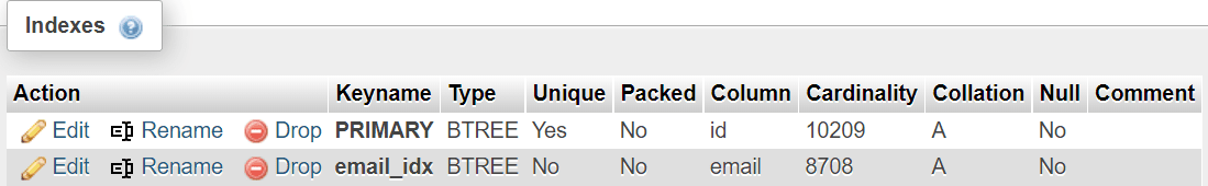

   
   

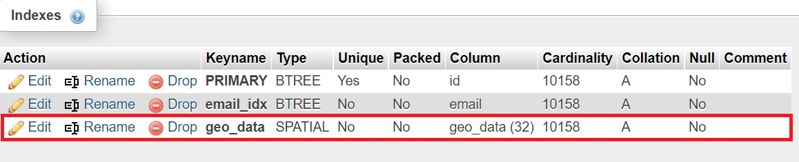
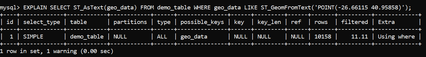
2. R-Tree, or spatial, indexes can only be defined on geographical data – that is, columns having the GEOMETRY data type. R-Tree indexes are suited for indexing geographical data due to its nature: the data structure is suited for geographical coordinates, but bear in mind that LIKE queries may not always use indexes as you can see below:
   ALTER TABLE 'demo_table' ADD SPATIAL INDEX(column);
For more detail on R-Tree structures, see this Wikipedia article.
   
3. For an index to be a covering index for a query, it must include all of the columns in a table that a specific query is using. So, for example, if our query looks like SELECT * FROM demo_table WHERE c1 = 'A' AND c2 = 'B';, our covering index would look like so (phpMyAdmin will also show the cardinality of both index key columns towards the right):
   ALTER TABLE `demo_table` ADD INDEX covering_idx (email,username);
   
   
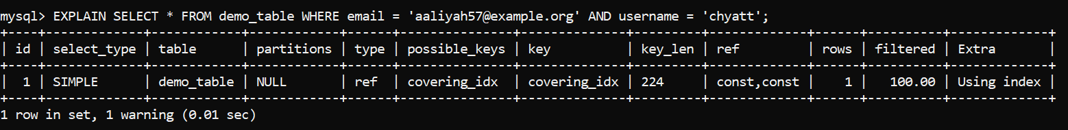
   In this case, MySQL has elected to use the covering index – the index is of 224 characters in size.
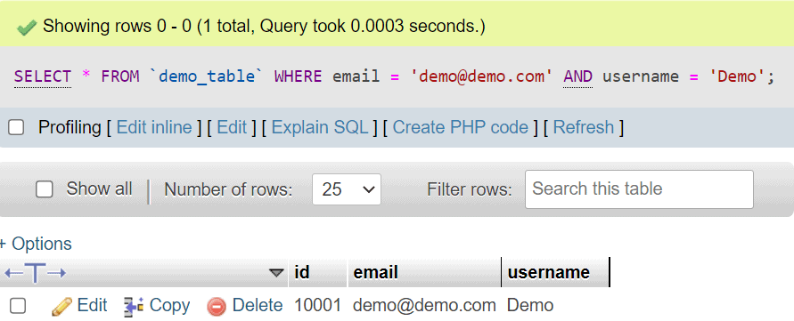
   Covering indexes cover all of the fields required for a query to execute (see example below.) A covering index covers all of the columns required for a query to execute, but not necessarily in a specific manner, meaning that if we would switch the order of columns, the index would still be covering. If our query looks like this, we would most likely benefit from an index on the columns c1, c2, and c3:
   SELECT * FROM demo_table WHERE c1 = ‘Demo’ AND c2 = 'Demo' AND c3 = 'demo@demo.com';

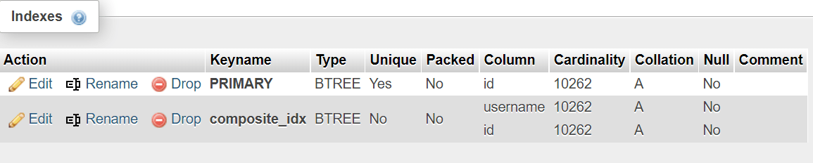
4. Composite indexes include multiple columns, but will not necessarily cover all of the columns for any given query. If we have three columns – c1, c2, and c3, a composite index would be any index that covers multiple columns. Such an index may cover columns c1 and c2, it may index the columns c3 and c1, it may have other combinations – but if the index does not cover all of the columns required for a query to execute, it’s not a covering index. Composite indexes are simply indexes that include multiple columns inside of them and they don’t have anything unique to themselves, other than the fact that key columns need to be ordered first, so the most important columns are scanned first.
   In this case, we cover the username and id columns with a query like so:
   ALTER TABLE 'demo_table' ADD INDEX covering_idx(username,id);

   
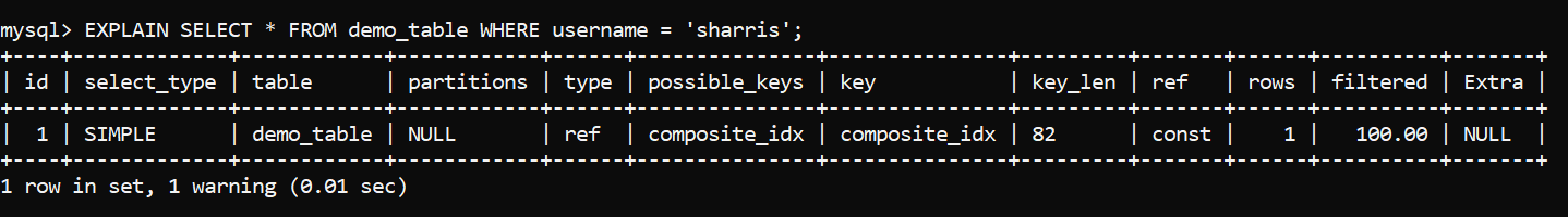
5. Indexing a prefix of a column might be a necessity to save storage space – the golden rule here is that the fewer characters that are in the prefix, the better for storage, but worse for performance because of the additional scan of rows that partially match that is necessitated. If you don’t have much storage space but still want increased performance, prefix indexes are for you. Define prefix indexes like so (in this example, we assume that your column is called c1 and we index the first 5 characters of the column):
   ALTER TABLE 'demo_table' ADD INDEX idx_name(c1(5));
When such indexes are in use, we could still search for exact matches as we do below (we only indexed the first 5 characters, but the query was still using index):
   
6. PRIMARY KEY indexes are usually defined when creating a table, and they must be set to increment automatically:
   CREATE TABLE demo_table (
'id' INT(255) PRIMARY KEY AUTO_INCREMENT,
`column_1` VARCHAR(255),
...
);
   
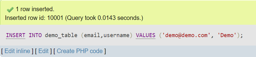
   As you can see from the query below, the id column has incremented by 1 since one row was inserted into the table:
   

As far as PRIMARY KEY constraint indexes are concerned, keep in mind that the type of the column that has a primary key doesn’t have to be an integer. For MySQL, PRIMARY KEY constraints have the following requirements:

• The column that has a primary key constraint on it cannot be null, nor should it be empty.
• The column that has a primary key constraint on it must only contain unique values.
• A table can only contain one primary key constraint.
• The length of the column that has a primary key constraint cannot be longer than 767 bytes.

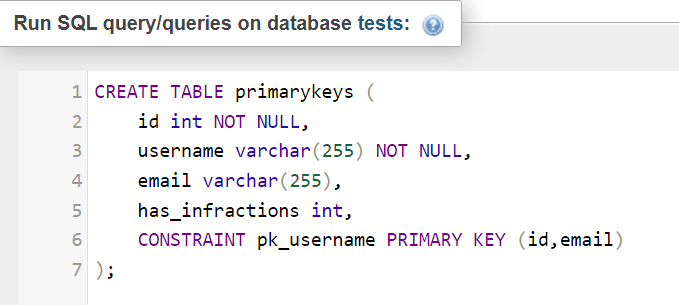
Also, keep in mind that primary key constraints can consist of multiple columns – for many, such an approach looks like the following (notice the constraint on line 6):

Indexes affect queries in various ways: the aim of B-Tree indexes is to help the database find rows matching a specific WHERE clause quickly enough. How much the performance is improved can depends on how our instances are configured. Some indexes are typically added when creating a table or with an ALTER TABLE query defined above.

There are also fulltext type indexes for those who would like to run more queries that behave more like search engine, for example when searching through long text columns, Fulltext indexes are defined by adding the FULLTEXT keyword in the ALTER TABLE or CREATE TABLE queries, or when creating tables, they can be defined like so:

There is also a type of index that’s a fit for the MEMORY storage engine – hash indexes can be defined like so (in this case, demo_table_memory is based upon the MEMORY storage engine instead of InnoDB. Make sure your table is based upon the MEMORY storage engine before running this query):
ALTER TABLE `demo_table_memory` ADD INDEX idx_name(column); USING HASH;
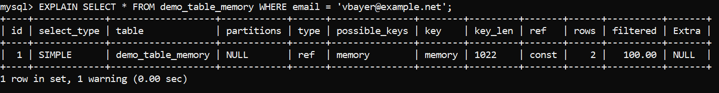
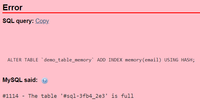
Hash indexes are only supported when the MEMORY storage engine is in use, and they only support exact matches of data (only queries with the “=” operator.) Also, note that you should bear in mind the amount of memory available on the server to not face the “The table is full” error (the name of the table will be weird because it’s in memory):

Partitioning MySQL

Now for partitions. They also have multiple types – aside from the fact that tables can be either partitioned horizontally or vertically, there are six partitioning types that are available. Also, mind the fact that since some storage engines don’t provide support for partitioning, partitions are recommended to use on InnoDB or XtraDB storage engines.

MySQL has six partitioning types (as of the time of writing, MySQL supports horizontal partitioning, but not vertical):

1. Partitioning by RANGE – such a partitioning type is used to partition data that falls within a given range. For example, if we have a large data set and we search for values beginning with numbers, we might benefit from partitions beginning with 0, 1, 2, and other numbers.
2. Partitioning by LIST – such a partitioning type is used to partition data that falls within one category in one partition, another category in another, etc. Think about geographical data falling in East, West, North, or East – such a partitioning type would be useful when 4 partitions are in use and values of rows could fall in one or more of defined lists.
3. Partitioning by COLUMNS can let people partition data by columns – i.e. such a partitioning type lets you use multiple columns as partitioning keys.
4. Partitioning by HASH is frequently used when partitioning id columns. Partitioning by HASH lets people split the data into a specified number of partitions with an equal amount of rows in them.
5. Partitioning by KEY is similar to partitioning by HASH, except that MySQL chooses the way of partitioning data. If users don’t want to, columns don’t have to be defined – simply specifying the number of partitions is enough.

The list below will tell you when certain partitioning types should be used:

• Partitioning by RANGE is frequently used by search engines that deal with a lot of data and need quick SELECT response times.
• Partitioning by LIST is used when we need a couple of lists falling within a category.
• Partitioning by COLUMNS is used by MySQL to determine which partitions are to be checked for matching rows or for the purpose of placing rows into partitions.
• Partitioning by HASH ensures even distribution of data across partitions.
• Partitioning by KEY is similar to partitioning by HASH, just that it takes a hashing function provided to it by MySQL.

There is also a concept known as subpartitioning which is relatively self-explanatory: it refers to partitions within partitions.

Partitions are usually defined when creating tables, and they can be defined like so (in this example, we use partitioning by KEY, but other partitioning types can be defined in a similar fashion – refer to the documentation for explanation, and before deciding on any one specific partitioning type, make sure to experiment):

In newer versions of MySQL (MySQL 8.0 and above – at the time of writing, MySQL 8.0.31 was the most recent stable release), partitioning is only supported in InnoDB and NDB storage engines – if older versions of MySQL are in use, users can also elect to partition data in the MyISAM storage engine. For more details of how partitioning impacts SELECT operations, refer to the MySQL documentation.

Tips & Tricks for Optimizing Read Operations

The optimization of SELECT operations using indexes is not a completely worry-free operation where you add a bunch of indexes and it all just works. Problems are an inevitable part of optimization operations, so we’ve also prepared a quick cheat sheet of tips & tricks that you can glance at and solve if not all, at least the majority of the problems you’re facing:

• Use normalization wherever possible – a properly normalized database is typically great for SELECT queries. This is because the lack of redundant data means less to be read. This has its limits based on instance capacity, number of rows, and how many tables are needed to answer queries, but it is almost always better to have a well normalized database.
• After creating an index, make sure that your queries use the indexes you have created for the queries that read data. Use EXPLAIN to allow MySQL to tell you what indexes are used and why (see examples we gave earlier on.) and adjust where necessary.
• Make use of the LIMIT clause where necessary and avoid using the “SELECT *” operator if possible – the less data you select, the faster your queries will become (the default limit of rows that are returned by MySQL is 200.)
• If possible, avoid overcomplicating your SELECT statements. Sometimes using too many OR expressions can mean that MySQL needs to use an index more than one time. It can be valuable to consider splitting a query into two queries, returning less results (use LIMIT), or selecting fewer columns to return (instead of using SELECT * use SELECT columnname, columnname2, etc.)
• If you find yourself using wildcards with the LIKE expression (a wildcard is the '%' operator), make sure to employ them only at the end of the search string. Using '%' at the start of your expression will return all data to be scanned, which typically makes the search operation slower.

SELECT Queries: DDL and the Data

As we’ve mentioned in the beginning of the article, now we’ll provide you with a couple of DDL operations to help you get started.

First off, we have to create the tables (the names of the tables and their contents can be any – also note that the tables should use the InnoDB or XtraDB storage engines for the best results in the optimization realm):

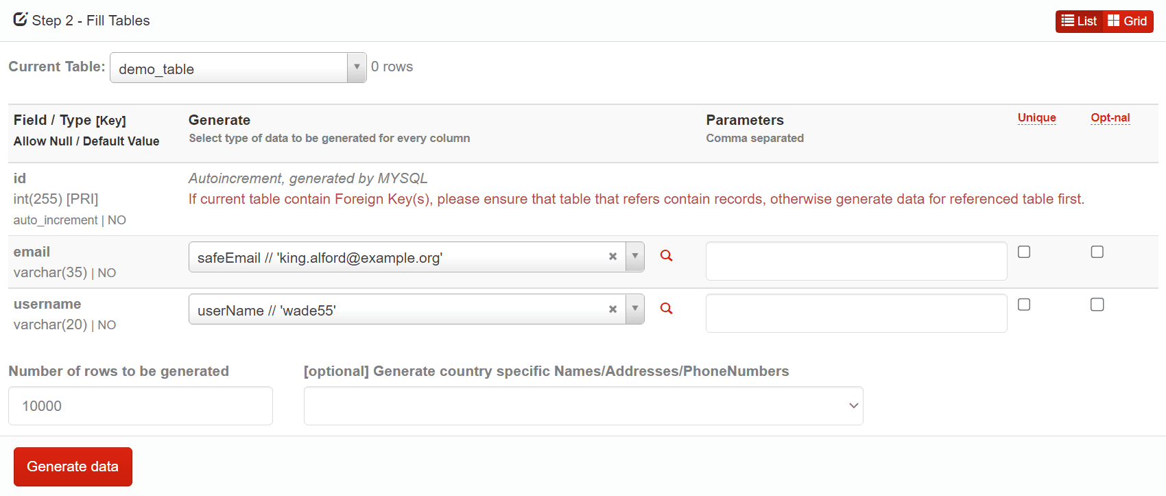
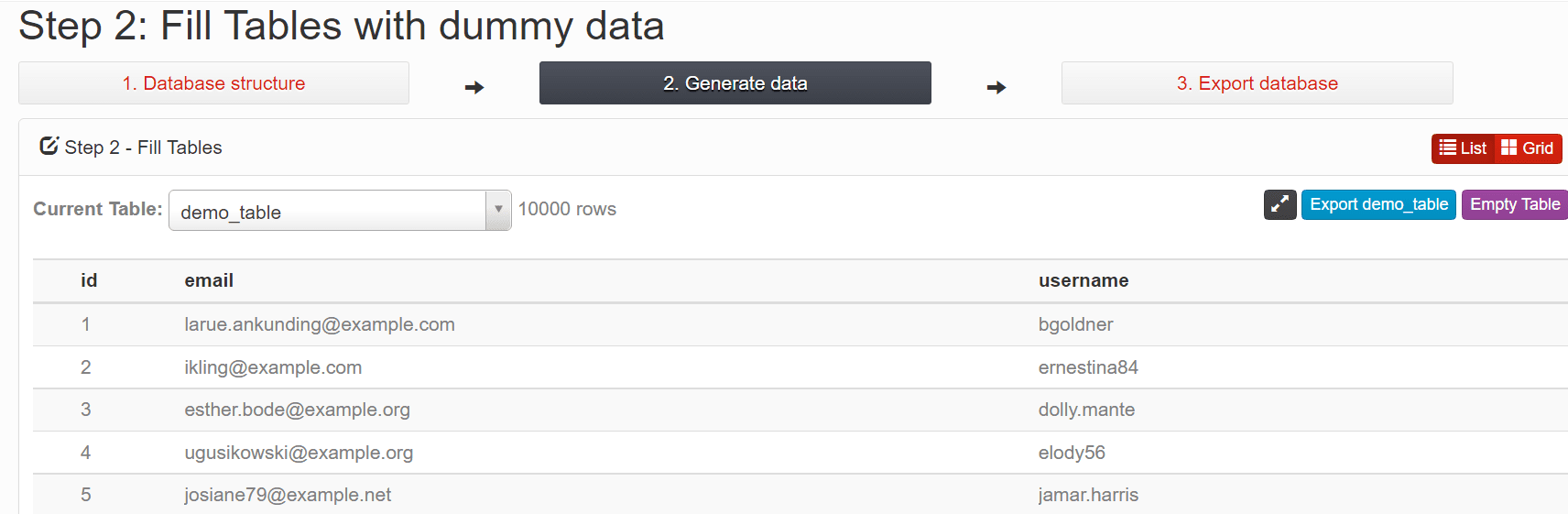
1. Now, we have to fill the table up with data – One method is to use the FillDB dummy data generator for that task – paste your database schema (you might need to rename some of your tables – the data generator saves all of the previously used table names), then generate data for columns:
   
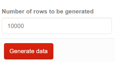
2. Finally, specify the number of rows to be generated (we recommend to generate no more than 100,000 rows at once to not overwhelm your browser), then move on:
   
3. Your data should be now ready to go – you will be able to view the data that the tool has generated:
   
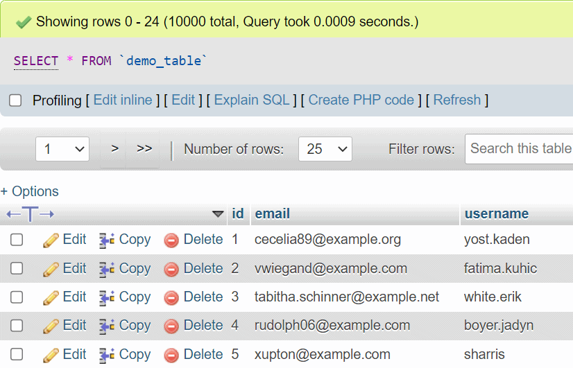
4. The only thing left for you to do is to import the data into your own database instance. Export the file from the dummy data generator by clicking the cyan button towards the right (it should say “Export tablename.”)
   

Now, import the data into MySQL via the CLI or the Import functionality within phpMyAdmin, and have fun optimizing your queries!

The Downsides of Optimizing SELECT statements

At the end of the day, almost everything we need to do to optimize a SELECT query comes down to the fact that we need to make MySQL able to access as little data as possible. If that doesn’t help, we need to look into the configuration of our MySQL instances.

However, one of the most significant nuances in this space is that when SELECT queries are being optimized, we need to compromise on storage and the performance of other queries.

That’s because indexes and partitions speed up read operations, but slow down the speed of INSERT, UPDATE, and DELETE queries. This is because when data is modified data also needs to be inserted, updated, or deleted together with it, and data may need to be shuffled around internally as well. It is rare that you have so many indexes that it noticeably harms performance, but it can happen, especially for high-throughput database applications.

Also keep in mind that the usefulness of indexes depends a lot on how frequently our queries are being executed. If a query is executed daily and saves 10 seconds on the runtime, is it worth it for all the maintenance it requires? Before making use of any advice mentioned in this article in a production environment, make sure to experiment and play around with the advice given in this article, and you should be good to go!

Summary

In this blog, we’ve walked you through numerous ways that help both novices and experienced DBAs optimize their SELECT query performance in MySQL. We’ve told you what query profiling has to do with their performance, walked you through the query execution plan provided by EXPLAIN queries, types of indexes, and partitioning.

We hope that some of the information provided in this blog has helped you optimize your SELECT query performance – tell us if the advice given in this blog has helped empower your applications in the comment section down below, come back to the blog to read up on how to optimize the performance of other types of queries, and until next time!