The series so far:

1. DAX financial functions: Loan calculations
2. DAX financial functions: Depreciation calculations

In this article, I will introduce the DAX financial functions. These 50-plus functions debuted around the time of the July 2020 release of Power BI Desktop. DAX financial functions are largely derived from those found in Excel, and so will seem familiar to many of you. A large number of this sizable number of functions are most useful in relatively specialized scenarios. I’ll be focusing, within this multi-part series, upon the more popular functions – popular because they concentrate upon lending, borrowing, and monitoring money, the lifeblood of virtually all business ventures.

Say you have a client who has contacted you to ask for an introduction to the new functions, preferring that you deliver quick overviews for the most popular, based upon the widespread use of their Excel counterparts. Because you agree that a “lunch-and-learn” format will be most accessible to the handful of Power BI authors in accounting and finance, you decide to parcel your introduction over short sessions, each of which will group a few related functions together, with practice examples based upon a small  dataset.

I’ll kick off this introduction with a small subset of the DAX financial functions that are used regularly within a popular area of analysis and reporting: the performance of calculations with loans. To this end, this article focuses upon the following DAX financial functions:

• PMT()
• RATE()
• NPER()
• PV()
• FV()

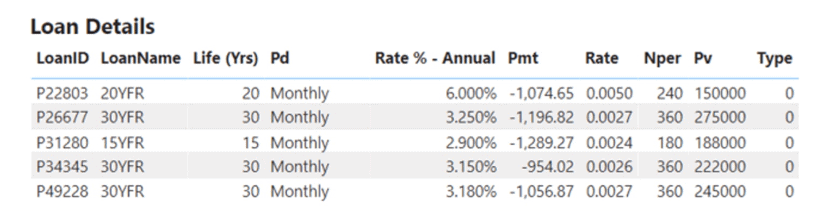
Illustration 1: The Focus in this Article is a Handful of Loan-Related Financial Functions

As a part of this introduction, you’ll have an opportunity to examine how each function can be employed to support business requirements of the sort that your hypothetical colleagues encounter routinely, and, for the most part, accomplish with Microsoft Excel, in meeting regular business requirements. You’ll learn the purpose of each function, and then undertake a practice example with each that demonstrates how it interacts with a small loan data set, via a calculation that you construct. Moreover, you will:

• Examine the syntax involved in exploiting the function.
• Undertake an illustrative example of the use of the function in a practice exercise.
• Review a brief discussion of the results you obtain in the steps of the practice example.

Preparation for the Practice Exercises in this Level

Assuming that you have installed Power BI Desktop (the illustrations in this article reflect the August 2020 release), you are ready to download and open the sample Power BI Desktop file. You will use the file for hands-on practice with the concepts introduced in the sections that follow.

NOTE: The latest version of Power BI is available for free download at www.powerbi.com.

Download and Open the Sample Power BI File (.pbix) for Use in this Article

The small sample Power BI file you’ll be using contains enough imported data to support practice exercises for the functions covered in this article. You’ll add the calculations and visualizations upon which the article focuses as you go. Using the sample dataset provided will ensure that the results you obtain in following the detailed steps of the exercises agree to the results obtained (and depicted) as you progress through the individual sections.

Once the sample .pbix file is downloaded, take the following steps to open it in Power BI Desktop.

1. Open Power BI Desktop.
2. Select File – Open other reports from the splash dialog that appears upon entry, as shown.

Illustration 2: Select Open Other Reports on the Splash Dialog that Appears

3. Navigate to the downloaded .pbix file.

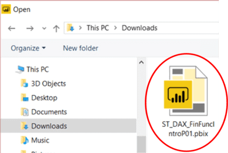
Illustration 3: Select the Downloaded File and Open …

4. Click Open.

The .pbix file opens, and you arrive within the Report view, which consists of a single tab containing a blank canvas. As many of you are aware, you can tell you are in the Report view because the current view (of the three views available in the upper left corner, Report, Data, and Model) is indicated by the yellow bar to the left of the icon.

5. Click the Data view icon along the left of Power BI Desktop, as desired, to become familiar with the basic sample model.

At this point, you’ll construct a table visualization to contain loan details to which you will need to be able to easily refer to create calculations using DAX financial functions in the practice examples. This table will also serve as a means of verifying your results for each of the calculations you create.

Construct a Table Visualization to Contain Loan Details for Reference and as an “Answer Key”

1. In the sample Power BI model, make sure to be in the Report view.
2. Click the cursor in the upper half the blank canvas.
3. Click the Table icon in the collection atop the Visualizations tab, to create a blank table on the canvas.

Illustration 4: Create a New Table Visualization on the Canvas

4. Ensuring that the above table visualization is selected, add the following fields (from the Loans table in the Fields pane) to the Values section of the Fields tab of the Visualizations pane:
   • LoanID
   • LoanName
   • Life (Yrs)
   • Pd
   • Rate % – Annual
   • Pmt
   • Rate
   • Nper
   • Pv
   • Type

The fields appear in the table as depicted.

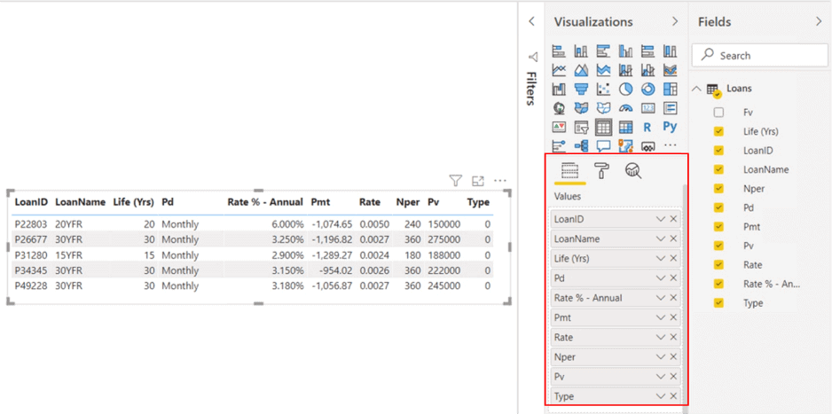
Illustration 5: Additions in the Values Section of the Fields Tab

Finally, it’s a good idea to label the table you’re are creating – as I’ve said throughout my Stairway to DAX and Power BI series and elsewhere. This is a minor point, but, as multiple visualizations tend to accumulate within a development environment, it is often helpful to make them easily distinguishable via descriptive, working titles. It’s also a great way to identify the at-a-glance verification mechanism for other internal team members to use, say, in granting approval to promote a model and its contents to production from development.

5. With the new table selected, once again, click the Format (paint roller) tab, underneath the visualizations collection atop the Visualizations pane.
6. Scroll down to the Title section of the Format settings.
7. Click the Title slider to On.
8. Expand the Title section by clicking the carat to the left of the Title label.
9. Type Loan Details in the Title text box.
10. Set formatting as desired (you can see what I used in the illustration below).

The settings for the Title section of the Format tab appear, alongside the new table, somewhat as depicted.

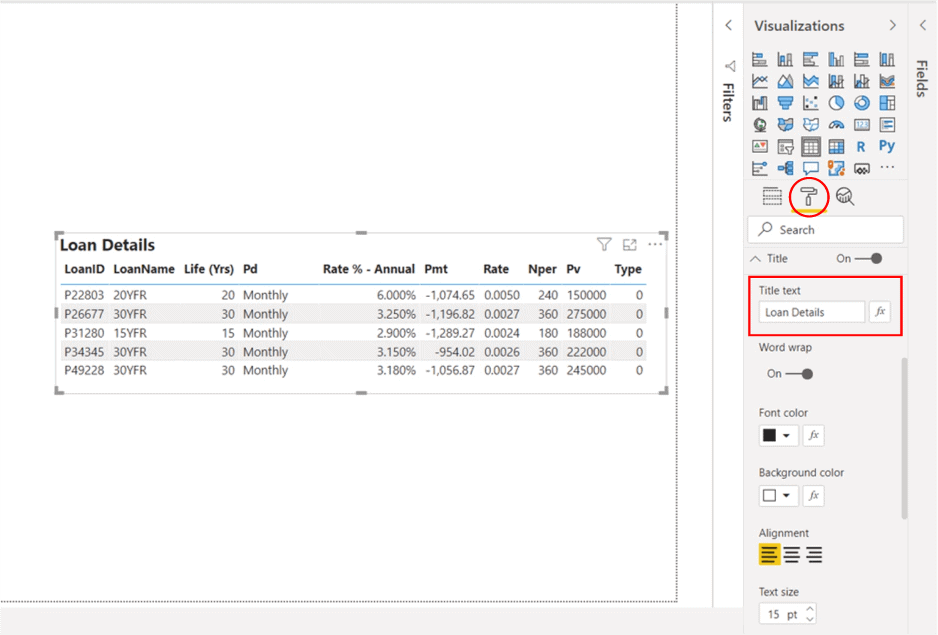
Illustration 6: Title Settings for the New Table

Finally, you can wrap up preparation for the practice exercises by constructing a table similar to the one above, to contain a calculation each for the DAX financial functions introduced in this article.

Construct a Second Table Visualization to Contain Calculations You Create within the Practice Example

You can use a quick “copy and customize” action to create a table to house your practice examples.

1. Click the table you created above on the canvas to select it.
2. Select CTRL+C (Copy) to copy the existing table visualization.
3. Click outside the table and onto the blank canvas.
4. Select CTRL + V (Paste) on the keyboard to create an identical copy of the table you just created.
5. Move the newly created copy above the original on the canvas to create working space, approximately as shown.

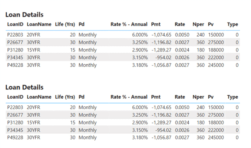
Illustration 7: Copied Table above the Original …

6. Ensuring that the new clone table (now above the original) remains selected on the canvas, deselect the following fields from the Values section of the Fields tab on the Visualizations tab to remove them from the new table visualization.
   • Pmt
   • Rate
   • Nper
   • Pv
   • Type

7. With the new table still selected, click the Format tab, once again, underneath the visualizations collection atop the Visualizations pane.
8. Scroll down to the Title section of the Format settings.
9. Expand the Title section by clicking the carat to the left of Title label.
10. Change the Title from Loan Details to DAX Finance Calculations (“c_”).
11. Leave formatting as is.

The clone table now appears, above the original table, as depicted.

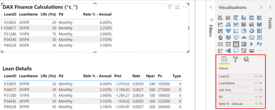
Illustration 8: The Clone becomes the Calculations Table …

You now have a destination container for the calculations you will create with each DAX financial function introduced in the sections below.

Shared Parameters for DAX Financial Functions in Part 1

The financial functions introduced in this article are related. As you are about to see (and as many of you already know), each function is an argument (parameter) within the others. The information supplied within the Loan Details table above reflects the parameters for each loan in the group contained within your Power BI source table.

Any one of these values can be computed via a DAX financial function using the other parameters. To gain an introduction to the operation of each function efficiently, you will work through a separate practice exercise for each function, where you can get hands-on exposure to the associated function as if it were missing from the data source, using the remaining parameters. As an example, you’ll employ the NPER() function by treating the Nper value in the table as missing, and calculating it with the remaining values, within the individual NPER() introduction and practice section.

For this reason, it makes sense to place an explanation of the shared arguments / parameters here, so as not to repeat them in the Syntax section of each function. Should you need to refresh your understanding of the meaning of any given argument, you need only refer to the below.

The shared arguments / parameters are:

• Rate – The interest rate per period.

Example: Say an individual takes out a 30-year mortgage loan for a primary residence at a 3.5 percent annual interest rate. Assuming regular monthly payments, the interest rate is .035 / 12, or .002917 per month. .002917 would be added into the formula as the Rate.

• Pmt – The payment made each period of, and which typically stays the same over, the life

of the annuity. This payment usually includes principal and interest but no other fees or taxes.

• Nper – The total number of payment periods in an annuity. (Error occurs if less than 1.)

Example: In the case of an individual taking out a 30-year mortgage loan with monthly payments, the number of payment periods would be 360 (30 years times 12 months). 360 would be added into the formula as Nper.

• Pv – The present value, or the total amount that a series of future payments is worth in

present time. Present value is often called “principal.”

Note: I get into present value in more depth in the discussion of the DAX PV() function below.

• Fv – (Optional) The future value, or cash balance one expects to attain after the last

payment is made (Fv is assumed to be blank, if omitted).

Example: Say an individual determines to save $ 20,000 for a project she expects to begin in 7 years. $ 20,000 represents the future value. She could estimate a conservative range for the interest rate available, and, based upon that, determine how much to save each month.

• Type – (Optional) The number 0 or 1. Type indicates when payments are due.

Accepted values:

• 0 (or blank) Payments are due at the end of the period
  •  
• 1 Payments are due at the beginning of the period

DAX Financial Function: PMT()

According to the Data Analysis Expressions (DAX) Reference, the PMT() function “calculates the payment for a loan based on constant payments and a constant interest rate.” PMT() is a highly popular function in Excel where finance professionals use it heavily in real estate and other lending modeling. Its underlying formula is the logic commonly found within loan payment calculators. PMT() calculates the payment made per period, for example, the monthly payment for a loan, or the monthly payment to an account set up to accumulate a savings goal.

The basic idea is that, supplied with an interest rate, a number of periods (months in the examples you encounter here) and the total (or “present,” in the case of a loan) value, you have what you need to calculate the amount of the individual payments for a typical loan. (And yes, the financial environment is full of many variations, minor to exotic, which are beyond the scope of this introductory article.)

Syntax

Syntactically, the parameters you provide are specified within the parentheses to the right of PMT as shown:

The arguments are explained in the section named Shared Parameters for DAX Financial Functions in Part 1 above.

Return Value and Further Remarks

PMT() returns a value that includes principle and interest only. Somewhat obviously, fees, taxes, insurance, reserve payments, and other costs associated with loans are computed and added outside this calculation.

Keep in mind that the units for Rate and Nper must be consistent.

Example: An individual makes annual payments on a 10-year loan, the annual interest rate for which is 6 percent. The Rate, of course, is .06, and the Nper is 10. If monthly payments are made for the same loan, Rate should be .06 / 12 (.005), and Nper is 10 x 12 (120).

You’ll get some hands-on practice with PMT() in Power BI in the next section.

Practice

The operation of PMT() will become clear using the data contained in the Power BI model you have downloaded and prepared above. You’ll begin with the dataset that appears in the model, and create a calculation that employs PMT(), whose parameters are selected out of the loans data in the table provided. Along with the other functions you examine in this article, the “answer” to be expected via the calculation you create will already exist in static form in the table within the model. It will also appear within the Loan Details table visualization that you created in the preparation steps. The functions within this article are largely dependent upon each other, as you will see – and this is a great way to “view all the cards simultaneously,” while observing how each function works in DAX.

Employ the DAX PMT() Function to Generate Basic Monthly Loan Payments

You can take the following steps to create a calculation to return payments for various loans in the sample dataset.

1. From the Report view, right click the Loans table in the Fields pane of the model.
2. Select New column from the context menu that appears.

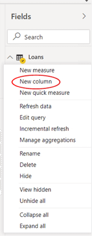
Illustration 9: Creating a New Calculation …

3. Type, or cut and paste, the following into the Formula bar:

The calculation appears as shown in the Formula bar:

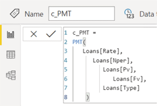
Illustration 10: Calculation Containing the PMT() Function …

4. Click the checkmark to the left of the Formula bar to check and commit the calculation, and to create the new calculated column.

The calculation c_PMT appears in the Loans table in the Fields pane.

NOTE: You will be naming the calculations you create in this article with a c_ prefix, perhaps somewhat obviously to leave their names very close to that of the DAX financial function they employ, while making them easily identifiable.

5. With the new calculated column c_PMT selected in the Fields pane, make the following Format settings underneath the main menu:
   • Currency ($)
   • 2 decimal places
   • Don’t summarize

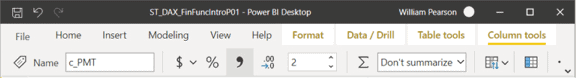
Illustration 11: Calculated Column Format Settings

6. Select the DAX Finance Calculations (“c_”) table visualization, once again, and add the new c_PMT calculation to the Values section of the Fields tab for the table, underneath the existing Rate % – Annual calculation.

The Pmt value within the Loan Details table visualization serves as a means of checking the output accuracy of the new calculation, as shown in the current results.

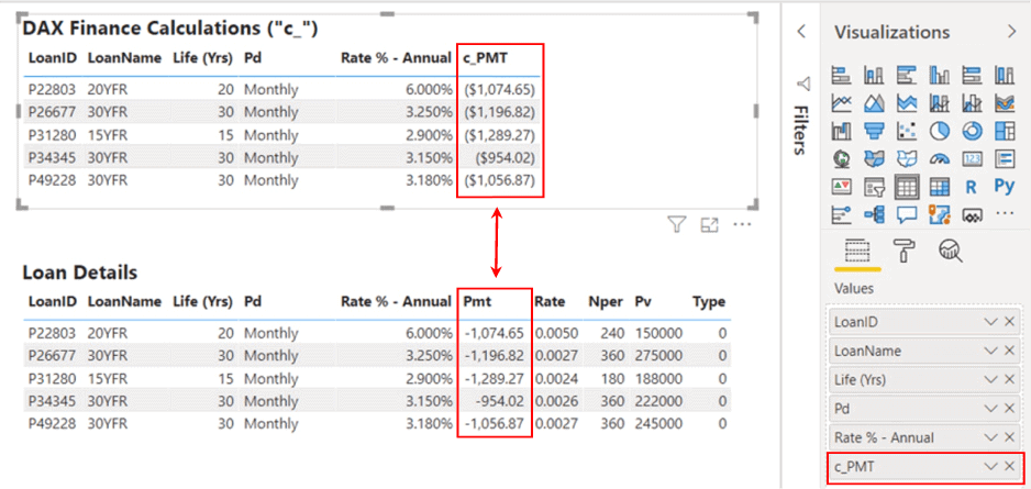
Illustration 12: Verifying Accuracy of Value Returned via the New Calculation

If you’ve obtained similar results to the above, you can conclude that you’ve successfully assembled a calculation to demonstrate the operation of the DAX PMT() financial function.

In the next section, you’ll be introduced to the DAX RATE() function.

DAX Financial Function: RATE()

According to the Data Analysis Expressions (DAX) Reference, the DAX RATE() financial function “returns the interest rate per period of an annuity.” RATE() can be used to calculate interest rates in scenarios ranging from determining the average annual rate of return one might earn from a bond purchased, to determining the percentage of amortization or depreciation per period, to calculating a given security’s yield to maturity – and many other settings in between. Two of the more common uses to which RATE() is put might involve determining the interest rate required by a loan of a given amount, or to reach a targeted amount on an investment, over a specific period of time.

You’ll take a look at how RATE() works with the loan data you used as a source in the PMT() section earlier. You’ll take up your practice with RATE() as if the rate itself is the only unknown variable, and use the RATE() function to calculate the periodic interest rate to pay off a stated present value, with an associated stated periodic payment for the loan, and with a stated total number of payments.

Syntax

Syntactically, the parameters you provide are specified within the parentheses to the right of RATE as shown:

The arguments are explained in the section named Shared Parameters for DAX Financial Functions in Part 1 above, with the exception of the Guess parameter, which only occurs in this function.

• Guess – (Optional) A guess as to what the rate will be.
  • • If omitted / blank, Guess is assumed to be 10%.
    • If Rate does not converge, attempt different values for Guess. Per the documentation, “Rate usually converges if Guess is between 0 and 1.” A practical approach might be to simply place Rate / Nper from the loan / other description into the Guess (leaving it blank has resulted in errors, in my experience, although the documentation states that Guess is “optional.”)

Return Value and Further Remarks

RATE() returns the interest rate per period, a value that includes principle and interest only.

Keep in mind that the units for specifying Guess and Nper must be consistent.

Rate and Nper must be consistent.

Example: An individual makes monthly payments on a 20-year loan, the annual interest rate for which is 6 percent. In this case, you would supply a Guess of .06/12, and 20*12 (or 240) for Nper.

Errors can be returned if the Rate, after 20 iterations, does not converge to within 0.0000001, or if a value of zero or less is supplied for Nper (unsurprisingly).

It’s time to get some hands-on exposure to RATE() in Power BI.

Practice

You will return to the Power BI model you’ve have prepared, and create a calculation in the Loans table that uses the RATE() function. The parameters, once again, for the function under examination, will be sourced from the Loans table within the model.

Recall that the answer to be expected via the calculation you create already exists in static form in the table within the model. The Loan Details table visualization that you created in the preparation steps contains this and other parameter values for easy visual validation.

Employ the DAX RATE() Function to Return the Monthly Interest Rates for a Group of Loans

You’ll create a calculation to return the respective periodic (monthly) interest rates for the loans in the sample dataset.

1. From the Report view, right-click the Loans table in the Fields pane of the model, once again.
2. Select New column from the context menu that appears, as you did earlier.
3. Type, or cut and paste, the following into the Formula bar:

The calculation appears as shown in the Formula bar:

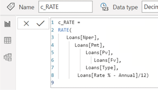
Illustration 13: Calculation Containing the RATE() Function …

4. Click the checkmark to the left of the Formula bar to check and commit the calculation, and to create the new calculated column.

The calculation c_RATE appears in the Loans table in the Fields pane.

5. With the new calculated column c_RATE selected in the Fields pane, make the following Format settings underneath the main menu:
   • Percentage (%)
   • 2 decimal places
   • Don’t summarize

6. Select the DAX Finance Calculations (“c_”) table visualization, once again, and add the new c_RATE calculation to the Values section of the Fields tab for the table, underneath the existing c_PMT calculation you added in the prior practice exercise.

The Rate value within the Loan Details table visualization serves as a means of checking the output accuracy of the new calculation, as shown in the current results.

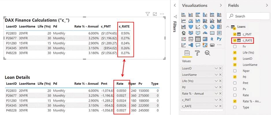
Illustration 14: Verifying Accuracy of Value Returned via the New Calculation

Again, you can conclude that you’ve successfully assembled a calculation to demonstrate the operation of the DAX RATE() financial function if your results agree to those above.

Next, you’ll get some exposure to the DAX NPER() function.

DAX Financial Function: NPER()

According to the Data Analysis Expressions (DAX) Reference, the DAX NPER() financial function “returns the number of periods for an investment based on periodic, constant payments and a constant interest rate.” NPER() is often used, within amortization or savings scenarios, to calculate points in time in which interest is earned/accrued. In this specific use case, it will calculate the number of periods to pay off a given loan under these circumstances – the total number of periods (months, quarters, years, etc.) over which the loan is to be paid.

You’ll see how NPER() works with the loan data in your Power BI model in the next section. Again, you’ll be working under the assumption that the parameter you seek, the number of periods, is the only unknown variable.

Syntax

Syntactically, the parameters to provide are specified within the parentheses to the right of NPER as shown:

The arguments are explained in the section named Shared Parameters for DAX Financial Functions in Part 1 above.

Return Value and Further Remarks

NPER() returns the number of periods in the life of a loan/investment.

Next, you’ll put NPER() to work upon the loan dataset within your Power BI model.

Practice

Once inside the Power BI model again, you’ll create a calculation in the Loans table that uses the NPER() function. The parameters, once again, will be sourced from the Loans table within the model. You’ll also be able to validate your results with NPER() instantly, via comparison of the calculated NPER() values to those in your Loan Details table visualization.

Employ the DAX NPER() Function to Return the Number of Periods for Each of a Group of Loans

Take the following steps to create another calculation, this time to return the respective number of periods in the lives of each of the loans in your sample dataset.

1. From the Report view, right-click the Loans table in the Fields pane of the model, once again.
2. Select New column from the context menu that appears, as before.
3. Type, or cut and paste, the following into the Formula bar:

 

The calculation appears as shown in the Formula bar:

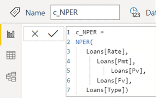
Illustration 15: Calculation Containing the NPER() Function …

4. Click the checkmark to the left of the Formula bar to check and commit the calculation, and to create the new calculated column.

The calculation c_NPER appears in the Loans table in the Fields pane.

5. With the new calculated column c_NPER selected in the Fields pane, make the following Format settings underneath the main menu:
   • Decimal number
   • 0 decimal places
   • Don’t summarize

6. Select the DAX Finance Calculations (“c_”) table visualization, once again, and add the new c_NPER calculation to the Values section of the Fields tab for the table, underneath the existing c_RATE calculation.

The NPer value within the Loan Details table visualization serves as a means of checking the output accuracy of the new calculation, as shown in the current results.

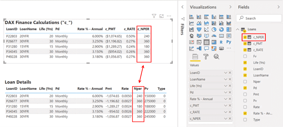
Illustration 16: Verifying Accuracy of Value Returned via the New Calculation

Each value displayed within your Loan Details table visualization should agree, once again, with that of the corresponding calculation in the DAX Finance Calculations table above.

In the next section, you’ll get some exposure to the DAX PV() function.

DAX Financial Function: PV()

According to the Data Analysis Expressions (DAX) Reference, the DAX PV() financial function “calculates the present value of a loan or an investment, based on a constant interest rate.” You have probably encountered the concept of present value (variously – and sometimes inconsistently – called “principal amount,” “present discounted value,” or even “discounted value”) in the business environment, or from exposure in finance or economics elsewhere.

PV() can be used with either a future value (say, an investment goal) or periodic, constant payments (as in the case of a mortgage loan). In the case of an investment, PV() returns the initial investment or deposit. For a loan, it calculates the amount one is borrowing. Because it represents the value of an anticipated income stream as of the date of valuation, the present value is almost always less than the future value (due to the time value/interest earning potential of money).

Syntax

Syntactically, the parameters you provide are specified within the parentheses to the right of PV as shown:

PV(<rate>, <nper>, <pmt>[, <fv>[, <type>]])

The arguments are explained in the section named Shared Parameters for DAX Financial Functions in Part 1 above.

Return Value

PV() returns the present value of a loan or investment.

Time to get some hands-on exposure to PV() in Power BI with the steps in the Practice section below.

Practice

Returning, once again, to the Power BI model you have prepared, you’ll create a calculation in the Loans table that uses the PV() function. As you’ve done with the preceding DAX financial functions, you’ll source the parameters for PV() from the Loans table within the model. Once again, the “answer” to be expected via the calculation you create already exists in static form in the table within the model. You can validate the results you obtain through easy comparison to the Pv column as displayed in the Loan Details table visualization that you created in your preparation steps.

Employ the DAX PV() Function to Return the Present Value for a Group of Loans

Create a calculation to return the respective present values for the loans in your sample dataset via the following steps.

1. From the Report view, right-click the Loans table in the Fields pane of the model.
2. Select New column from the context menu that appears.
3. Type, or cut and paste, the following into the Formula bar:

The calculation appears as shown in the Formula bar:

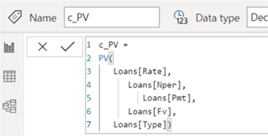
Illustration 17: Calculation Containing the PV() Function …

4. Click the checkmark to the left of the Formula bar to check and commit the calculation, and to create the new calculated column.

The calculation c_PV appears in the Loans table in the Fields pane.

5. With the new calculated column c_PV selected in the Fields pane, make the following Format settings underneath the main menu:
   • Currency ($)
   • 0 decimal places
   • Don’t summarize

6. With the DAX Finance Calculations (“c_”) table visualization selected, once again, add the new c_PV calculation to the Values section of the Fields tab for the table, underneath the existing c_NPER calculation.

The Pv value within the Loan Details table visualization serves as a means of checking the output accuracy of the new calculation, as shown in the current results.

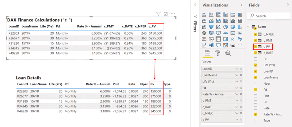
Illustration 18: Verifying Accuracy of Value Returned via the New Calculation

Again, verify the results you’ve generated to the corresponding values in the Loan Details table to ensure accuracy.

Finally, you’ll wrap the first part of “Introduction to DAX financial Functions” with an overview and demonstration of the DAX FV() function.

DAX Financial Function: FV()

According to the Data Analysis Expressions (DAX) Reference, the DAX FV() financial function “calculates the future value of an investment based on a constant interest rate.” FV() can be used to calculate future value in scenarios involving periodic, constant payments (as you’ve encountered within the loan-based data you’ve worked with throughout this article), and/or single “lump sum” payments. It reflects the principal plus interest received or paid.

Conceptually, future value is the value of an asset at a specific date in the future – what, for instance, a given sum of money today is worth at a specified future time, assuming a certain rate of return/interest rate. It is typically a consideration that arises in “time value of money” concerns, where it is easy to see the value of being able to determine how much money one will have at a future point, given, say, a starting balance, regular payments, and a compounding interest rate. Other factors, such as adjustments for inflation, are not taken into consideration within calculations one undertakes solely with FV().

You’ll take a look at how FV() works with the loan data you’ve have used within the other financial functions. You’ll take up your practice with FV() as if the future value itself is the only unknown variable, and use the FV() function to calculate the future value, with the associated stated parameters that are assigned for the respective loan.

Syntax

Syntactically, the parameters to provide are specified within the parentheses to the right of FV as shown:

The arguments are explained in the section named Shared Parameters for DAX Financial Functions in Part 1 above.

Return Value and Further Remarks

FV() returns the future value of an investment.

Keep in mind that the units for specifying Rate and Nper must be consistent.

Example: An individual makes monthly payments on a 20-year loan, the annual interest rate for which is 6 percent. In this case, you would supply a Rate of .06/12, and 20*12 (or 240) for Nper.

Now for some hands-on exposure to FV() in Power BI.

Practice

You’ll create a calculation in the Loans table once again, this time containing the FV() function and again sourcing the Loans table for the parameters.

Employ the DAX FV() Function to Return the Future Value for a Group of Loans

Create a calculation to return the future values for each of the loans in the sample dataset via the following steps.

1. From the Report view, right-click the Loans table in the Fields pane of the model, once again.
2. Select New column from the context menu once more.
3. Type, or cut and paste, the following into the Formula bar:

The calculation appears as shown in the Formula bar:

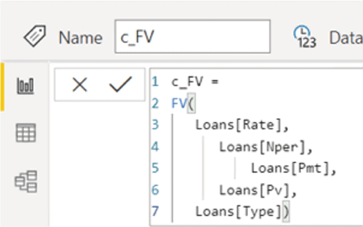
Illustration 19: Calculation Containing the FV() Function …

4. Click the checkmark to the left of the Formula bar to check and commit the calculation, and to create the new calculated column.

The calculation c_FV appears in the Loans table in the Fields pane.

5. With the new calculated column c_FV selected in the Fields pane, make the following Format settings underneath the main menu:
   • Currency ($)
   • 0 decimal places
   • Don’t summarize

6. Select the DAX Finance Calculations (“c_”) table visualization, once again, and add the new c_FV calculation to the Values section of the Fields tab for the table, underneath the existing c_PV calculation.

Future Value is not represented within the Loan Details table, but you can conclude that the output accuracy of the new c_Fv calculation is accurate, as the “future value” of a loan fully paid off, at the rate and number of periods specified, would near-zero (there would likely be minor rounding due to decimalization, etc.).

Summary

In this, Part 1 of an article series introducing the new DAX financial functions, I introduced a popular subgroup of those functions that deal largely with loans or investments. My objective was to examine how each function can be employed, within Power BI, to support analysis and reporting of the sort one might accomplish using Microsoft Excel. For each function you explored, you learned its purpose, then examined the DAX syntax involved in its use. Moreover, you gained exposure, via an illustrative example for each function, to the use of the respective function with practice loan data, and then confirmed your understanding of the results you had obtained with each function.

In Part 2 of this series, I will introduce a second group of the new DAX financial functions, this time the ever-popular Depreciation functions.