This article is part of Robert Sheldon's continuing series on Learning MySQL. To see all of the items in the series, click here.
As with many relational database management systems, MySQL provides a variety of methods for combining data in a data manipulation language (DML) statement. You can join multiple tables in a single query or add subqueries that pull data in from other tables. You can also access views and temporary tables from within a statement, often along with permanent tables.
MySQL also offers another valuable tool for working with data—the common table expression (CTE). A CTE is a named result set that you define in a WITH clause. The WITH clause is associated with a single DML statement but is created outside the statement. However, only that statement can access the result set.
In some cases, you can include a CTE with a SELECT statement that is embedded in another statement, as in the case of a subquery or a DELETE…SELECT statement. But even then, the WITH clause is defined outside of that SELECT statement, and only that SELECT statement can access the result set.
One way to think of a CTE is as a type of view with a very limited scope (one statement). Another way to think of a CTE is as a type of named subquery that is defined in a clause separate from the main query. However, a CTE is neither of these, and in this article, I explain how the CTE works and walk you through a number of examples that demonstrate the different ways you can use them to retrieve data.
Note: the examples use the tables and data that is created in the last section of the article titled: “Appendix: Preparing the demo objects and data”.
Getting started with common table expressions
A common table expression is defined inside a WITH clause. The clause precedes the main DML statement, which is sometimes referred to as the top-level statement. In addition, the clause can contain one or more CTE definitions, as shown in the following syntax:
|
1 2 3 4 |
WITH [RECURSIVE] cte_name [(col_name [, col_name] ...)] AS (select_query) [, cte_name [(col_name [, col_name] ...)] AS (select_query)] ... top_level_statement; |
If the WITH clause contains more than one CTE, you must separate them with commas, and you must assign a unique name to each CTE, although this applies only within the context of the WITH clause. For example, two SELECT statements can include CTEs with the same name because a CTE is limited to the scope of its associated top-level statement.
The CTE name is followed by one or more optional column names, then the AS keyword, and finally a SELECT query enclosed in parentheses. If you specify column names, their number must match the number of columns returned by the SELECT query. If you don’t specify column names, the column names returned by the SELECT query are used.
Common table expressions are typically used with SELECT statements. However, you can also use them with UPDATE and DELETE statements, following the same syntax as shown above. In addition, you can include CTEs with your subqueries when passing them into your outer statements. You can also use CTEs in statements that support the use of SELECT as part of the statement definition. For example, you can add a WITH clause to the SELECT query in an INSERT…SELECT statement or in a CREATE TABLE…SELECT statement.
For this article, I focus primarily on creating CTEs that use SELECT statements as their top-level statements because this is the most common way to use a CTE. This approach is also a good way to start learning about CTEs without putting any data at risk. You can then apply the fundamental principles you learn here to other types of statements as you become more comfortable with how CTEs work.
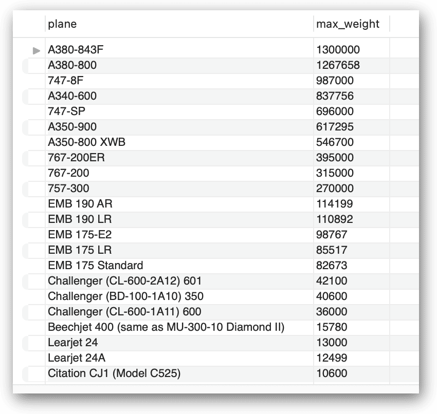
With that in mind, let’s start with a simple example. The following SELECT statement includes a WITH clause that defines a CTE named planes:
|
1 2 3 4 5 6 |
WITH planes AS (SELECT plane, engine_count, max_weight FROM airplanes WHERE engine_type = 'jet'); SELECT plane, max_weight FROM planes ORDER BY max_weight DESC; |
The SELECT query in the CTE retrieves all the planes in the airplanes table that have jet as the engine_type. The CTE’s result set is made up of the data returned by the SELECT query and can be accessed by the top-level SELECT statement.
The top-level statement retrieves the data directly from the CTE, similar to how a statement might retrieve data from a view. The main difference is that the view definition is persisted to the database and can be used by anyone with adequate privileges. The CTE, on the other hand, has a very limited scope and can be accessed only within the context of the top-level statement.
In this case, the top-level SELECT statement retrieves only the plane and max_weight columns from the CTE and orders the results by the max_weight column, in descending order. The following figure shows the results returned by the statement.
Of course, you can easily achieve the same results without the use of a CTE by querying the airplanes table directly:
|
1 2 3 4 |
SELECT plane, max_weight FROM airplanes WHERE engine_type = 'jet' ORDER BY max_weight DESC; |
However, I wanted to demonstrate the basic components that go into a CTE and how you can access that CTE from within the top-level SELECT statement. Both the CTE and top-level statement can certainly be much more complex—and usually are—but the principles remain the same.
Working with CTEs in the top-level SELECT statement
As mentioned earlier, a CTE is basically a named result set. When you query the CTE from within the top-level statement, the data is returned in a tabular format, similar to what you get when you query a view, permanent table, temporary table, or derived table (such as that produced by a subquery in a SELECT statement’s FROM clause). This means that you can work with the CTE in much the same way as you can those other object types. For example, one common approach to referencing a CTE within the top-level query is to join it with another table, as in the following example:
|
1 2 3 4 5 6 7 |
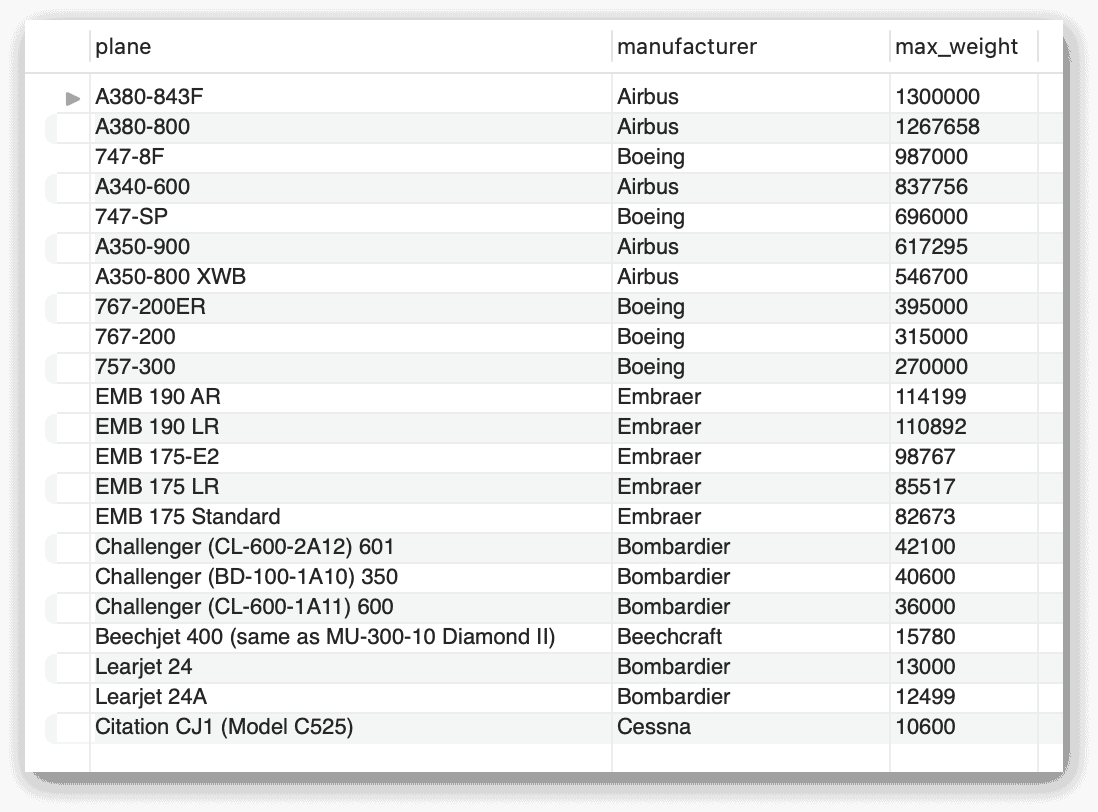
WITH mfcs AS (SELECT manufacturer_id, manufacturer FROM manufacturers) SELECT a.plane, m.manufacturer, a.max_weight FROM airplanes a INNER JOIN mfcs m ON a.manufacturer_id = m.manufacturer_id WHERE a.engine_type = 'jet' ORDER BY a.max_weight DESC; |
The WITH clause defines a single CTE named mfcs. The CTE’s SELECT query returns the manufacturer_id and manufacturer values from the manufacturers table. The top-level SELECT statement then joins the airplanes table to the mfcs CTE, based on the manufacturer_id column in each one. The following figure shows the statement’s results.
As this example demonstrates, you can treat the CTE much like any other table structure in your top-level query. However, just as you saw earlier, you can also recast this statement without a CTE by joining the airplanes table directly to the manufacturers table:
|
1 2 3 4 5 |
SELECT a.plane, m.manufacturer, a.max_weight FROM airplanes a INNER JOIN manufacturers m ON a.manufacturer_id = m.manufacturer_id WHERE a.engine_type = 'jet' ORDER BY a.max_weight DESC; |
Because there is so little data, the difference in performance between the two statements is negligible, but that might not be the case with a much larger data set. However, as is often the case with MySQL, it can be difficult to know which approach is best without running both statements against a realistic data set. Even then there might not be a significant difference in performance, in which case, it might come down to developer preference.
As noted earlier, MySQL often supports multiple ways to achieve the same results, as the preceding examples demonstrate. Common table expressions can sometimes help simplify code and make it more readable, which is a big point in its favor, but performance should generally be the overriding consideration.
Comparing different approaches usually requires that you test them on a valid data set, in part, because it can be difficult to find specific recommendations when comparing approaches. Not many database developers, for example, would be willing to say that you should always use CTEs rather than inner joins in all circumstances, or vice versa.
That said, you might come across recommendations that are less rigid and are perhaps worth considering, such as when comparing CTEs with subqueries. For instance, a CTE is often considered to be a better option if your SELECT statement includes multiple subqueries retrieving the same data, as in the following example:
|
1 2 3 4 5 6 7 8 9 |
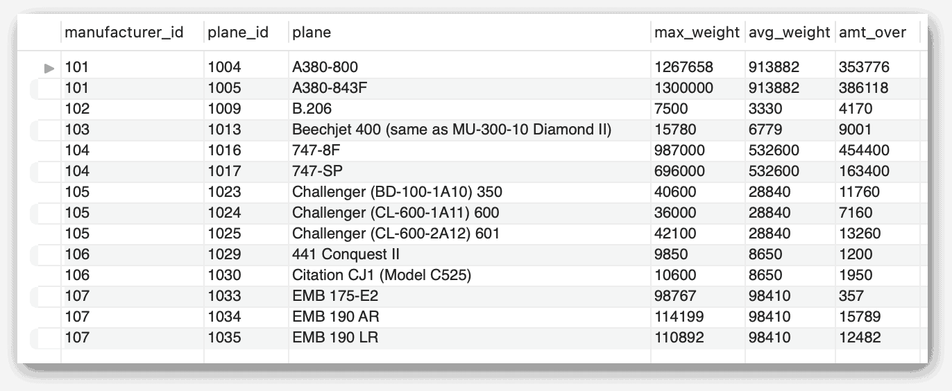
SELECT manufacturer_id, plane_id, plane, max_weight, (SELECT ROUND(AVG(max_weight)) FROM airplanes a2 WHERE a.manufacturer_id = a2.manufacturer_id) AS avg_weight, (max_weight - (SELECT ROUND(AVG(max_weight)) FROM airplanes a2 WHERE a.manufacturer_id = a2.manufacturer_id)) AS amt_over FROM airplanes a WHERE max_weight > (SELECT ROUND(AVG(max_weight)) FROM airplanes a2 WHERE a.manufacturer_id = a2.manufacturer_id); |
If this statement looks familiar to you, that’s because I pulled it from my previous article in this series, which covers subqueries. As you can see, the statement includes three subqueries, all of them the same, which can result in a fair amount of redundant processing effort, depending on how the database engine chooses to handle the query. The following figure shows the results returned by this statement.
Instead of using subqueries, you can achieve the same results by defining a CTE that retrieves the average max_weight value for each manufacturer. Then, in your top-level query, you can join the airplanes table to the CTE, basing the join on the manufacturer IDs, as shown in the following example:
|
1 2 3 4 5 6 7 8 9 |
WITH mfc_weights (id, avg_weight) AS (SELECT manufacturer_id, ROUND(AVG(max_weight)) FROM airplanes GROUP BY manufacturer_id) SELECT a.manufacturer_id, a.plane_id, a.plane, a.max_weight, m.avg_weight, (a.max_weight - m.avg_weight) AS amt_over FROM airplanes a INNER JOIN mfc_weights m ON a.manufacturer_id = m.id WHERE max_weight > m.avg_weight; |
In this case, the CTE specifies the column names to use for the result set, so the manufacturer_id values are returned as the id column. Additionally, the CTE groups the data in the manufacturers table by the manufacturer_id values and provides the average avg_weight value for each one.
The top-level query then joins the airplanes table to the CTE but limits the results to those airplanes with a max_weight value greater than the average weight returned by the CTE. Notice that, in place of the subqueries, the statement now uses the avg_weight column from the CTE.
Once again, the performance difference between these two approaches is negligible because we’re working with such a small data set. Only by running the statements against a more realist data set can we get a true picture of their performance differences. In my opinion, however, the CTE makes the code more readable, that is, it’s easier to follow the statement’s logic.
Defining multiple CTEs in one WITH clause
Up to this point, the examples in this article included only one CTE per WITH clause, but you can define multiple CTEs and reference any of them in your top-level statement. Just make sure that you assign different names to the CTEs and separate them with commas. For example, the following WITH clause defines three CTEs, which are all referenced in the top-level SELECT statement:
|
1 2 3 4 5 6 7 8 9 10 11 12 13 14 15 |
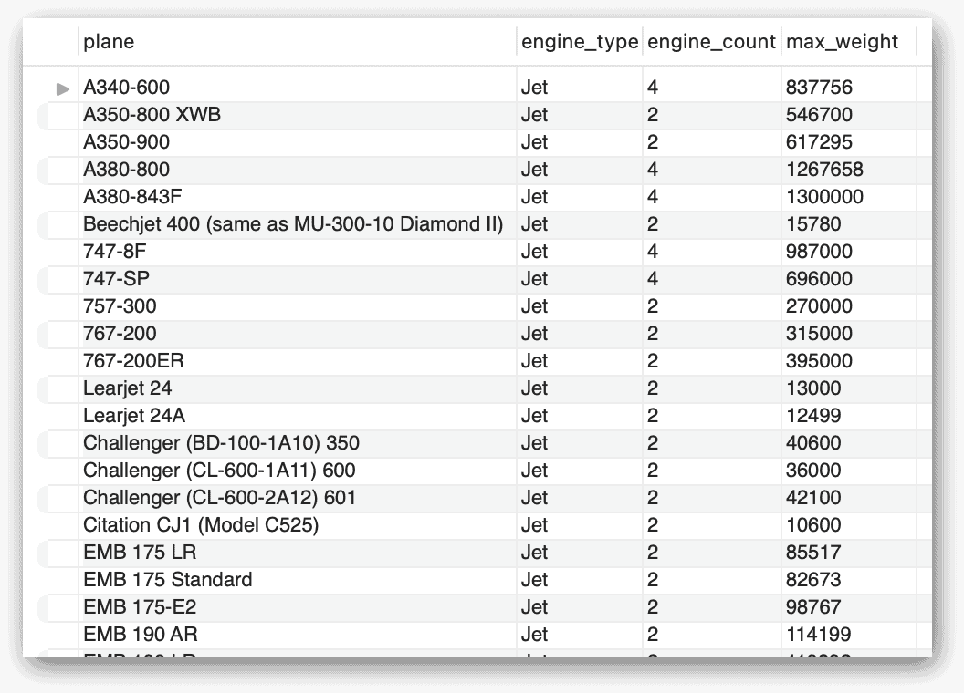
WITH jets AS (SELECT plane, engine_type, engine_count, max_weight FROM airplanes WHERE engine_type = 'jet'), turbos AS (SELECT plane, engine_type, engine_count, max_weight FROM airplanes WHERE engine_type = 'turboprop'), pistons AS (SELECT plane, engine_type, engine_count, max_weight FROM airplanes WHERE engine_type = 'piston') SELECT * FROM jets UNION ALL SELECT * FROM turbos UNION ALL SELECT * FROM pistons; |
The three CTEs are similar except that they each pull data based on a different engine_type value. The top-level SELECT query then uses the UNION operator to join them altogether. (The UNION ALL operator combines the results from multiple SELECT statements into a single result set.) The following figures shows part of the results returned by this statement.
This is a fairly basic example, but it demonstrates the concept of defining multiple CTEs and referencing them in the top-level query. In this case, the three CTEs operate independently of each other, but you don’t always have to take this approach. For instance, the WITH clause in the following example also includes three CTEs, but in this case, the second CTE (mfc_avg) references the first CTE (mfcs), while the third CTE (pl_avg) stands alone:
|
1 2 3 4 5 6 7 8 9 10 11 12 13 |
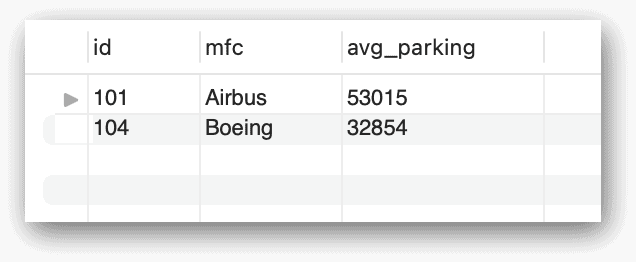
WITH mfcs (id, mfc) AS (SELECT manufacturer_id, manufacturer FROM manufacturers), mfc_avg (id, mfc, avg_parking) AS (SELECT m.id, m.mfc, ROUND(AVG(a.parking_area)) FROM mfcs m INNER JOIN airplanes a ON m.id = a.manufacturer_id GROUP BY manufacturer_id), pl_avg (avg_all) AS (SELECT ROUND(AVG(parking_area)) FROM airplanes) SELECT id, mfc, avg_parking FROM mfc_avg m WHERE avg_parking > (SELECT avg_all FROM pl_avg); |
As this example demonstrates, a CTE can reference a CTE that comes before it. However, this works in one direction only; a CTE cannot reference one that comes after it. In this case, the mfc_avg CTE joins the airplanes table to the mfcs CTE and groups the data based on the manufacturer_id value. The top-level query then retrieves data from this CTE, but returns only those rows with an avg_parking value greater than the average returned by the pl_avg CTE. The following figure shows the results returned by this statement.
Something worth emphasizing is that the WHERE clause in the top-level query includes a subquery that retrieves data from the pl_avg CTE. Not only does this point to the inherent flexibility of CTEs, but also to the fact that CTEs and subqueries are not mutually exclusive.
Working with recursive CTEs
One of the most useful aspects of the CTE is its ability to perform recursive queries. This type of CTE—known as the recursive CTE—is one that references itself within the CTE’s query. The WITH clause in a recursive CTE must include the RECURSIVE keyword, and the CTE’s query must include two parts that are separated by the UNION operator. The first (nonrecursive) part populates an initial row of data, and the second (recursive) part carries out the actual recursion based on that first row. Only the recursive part can refer to the CTE itself.
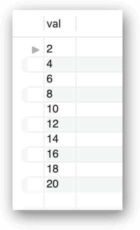
To help understand how this work, consider the following example, which generates a list of even numbers up to and including 20:
|
1 2 3 4 5 |
WITH RECURSIVE counter (val) AS (SELECT 2 UNION ALL SELECT val + 2 FROM counter WHERE val < 20) SELECT * FROM counter; |
The name of the CTE is counter, and it returns only the val column. The nonrecursive part of the CTE’s query sets the value of the first row as 2, which is assigned to the val column. The recursive part of the query retrieves the data from the CTE but increments the val column by 2 with each iteration. The query continues to increment the val column by 2 as long as val is less than 20. The top-level SELECT statement then retrieves the data from the CTE, returning the results shown in the following figure.
Note: Since the recursive query says < 20, you might be inclined to think it would not return 20 in the output. But the iteration that returns 20 does occur, but it stops iterating because the value is not less than 20 anymore.
When building a recursive CTE, be aware that MySQL places several limitations on the recursive part. The second SELECT statement cannot contain aggregate functions, window functions, the DISTINCT keyword, or the GROUP BY or ORDER BY clause.
Performing a recursive query can be useful when working with hierarchical data. To demonstrate how this works, I used the following code to create and populate a table named airline_emps, which stores the IDs and job titles for a group of fictitious employees, along with the ID of the person each one reports to:
|
1 2 3 4 5 6 7 8 9 10 11 12 13 14 15 16 17 18 19 20 21 22 23 24 25 26 27 28 |
CREATE TABLE airline_emps ( emp_id INT UNSIGNED NOT NULL, job_title varchar(50) NOT NULL, reports_to INT UNSIGNED NULL, create_date TIMESTAMP NOT NULL DEFAULT CURRENT_TIMESTAMP, last_update TIMESTAMP NOT NULL DEFAULT CURRENT_TIMESTAMP ON UPDATE CURRENT_TIMESTAMP, PRIMARY KEY (emp_id), CONSTRAINT fk_emp_id FOREIGN KEY (reports_to) REFERENCES airline_emps (emp_id) ); INSERT INTO airline_emps (emp_id, job_title, reports_to) VALUES (1, 'big boss', NULL), (2, 'divsional boss', 1), (3, 'supervisor', 2), (4, 'chief', 2), (5, 'designer', 3), (6, 'top exec', 1), (7, 'overseer', 6), (8, 'team leader', 6), (9, 'organizer', 8), (10, 'controller', 8), (11, 'specialist', 10), (12, 'analyst', 9); SELECT * FROM airline_emps; |
Everyone except for emp_id 1 (big boss) reports to another individual. For example, the overseer reports to the top exec, who in turn reports to the big boss. I included a SELECT statement along with the INSERT statement so you can verify the data after it’s been added to the table.
With this data in place, you can now create the following recursive CTE, which finds each person’s position level in the company and how that position fits into the reporting hierarchy:
|
1 2 3 4 5 6 7 8 9 10 11 12 13 |
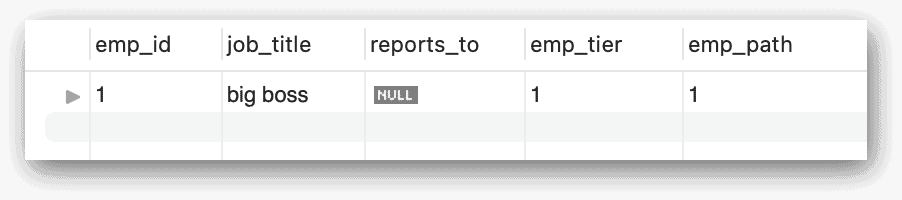
WITH RECURSIVE emps AS (SELECT emp_id, job_title, reports_to, 1 AS emp_tier, CAST(emp_id AS CHAR(50)) AS emp_path FROM airline_emps WHERE reports_to IS NULL UNION ALL SELECT a.emp_id, a.job_title, a.reports_to, e.emp_tier + 1, CONCAT(a.emp_id, ' / ', e.emp_path) FROM airline_emps a INNER JOIN emps e ON a.reports_to = e.emp_id) SELECT * FROM emps ORDER BY emp_tier, emp_id; |
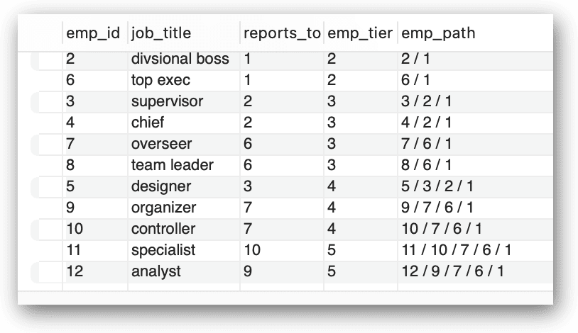
Because this is a recursive CTE, it is separated in two parts that are connected with the UNION ALL operator. The nonrecursive part populates the first row, based on the NULL value in the reports_to column. This row is for the big boss, who is at the top of the hierarchy. The nonrecursive part also assigns the value 1 to the emp_tier column and assigns the emp_id value to the emp_path column, converting the value to the CHAR data type. The first row returned by the CTE looks similar to that shown in the following figure.
The recursive part of the CTE uses an inner join to match the airline_emps table to the emps CTE. The join is based on the reports_to column in the airline_emps table and the emp_id column in the emps CTE. The join condition makes it possible to recurse through each level of the reporting hierarchy, based on the reports_to value. The recursive part then increments the emp_tier column by 1 with each new level in the hierarchy.
For example, emp_id 2 (divisional boss) and emp_id 6 (top exec) both report directly to emp_id 1 (big boss), so the emp_tier column for these two rows is incremented by 1, resulting in a value of 2 for each row. This means that they’re both in the second tier of the employee hierarchy. The next layer in the hierarchy are those individuals who report to the divisional boss or top exec, so the emp_tier column for these rows is set to 3. This process continues until there are no tiers left.
During this process, the emp_path column is also updated in each row by concatenating the emp_id vales to provide a representation of the reporting hierarchy. For instance, the reports_to column for emp_id 9 will show that the organizer reports to emp_id 8 (team leader), who reports to emp_id 6 (top exec), who reports to emp_id 1 (big boss), with each layer separated by a forward slash. The following figure shows the data returned by the query.
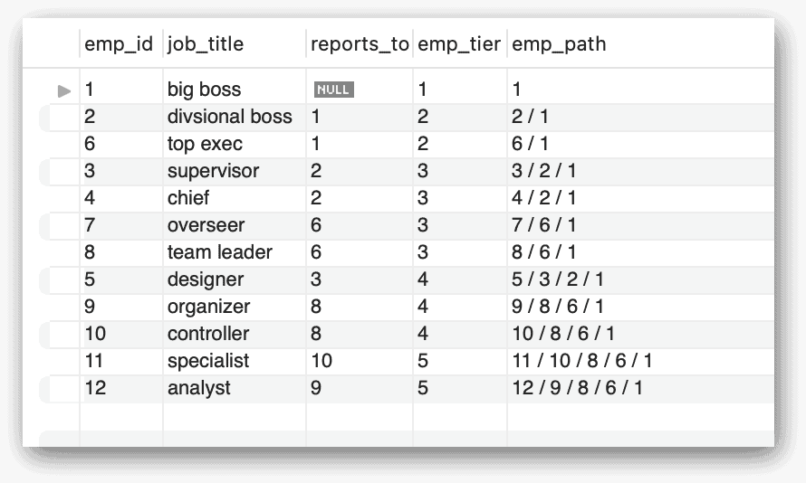
The top-level SELECT statement retrieves data only from the CTE, without joining to any other tables. The statement also includes an ORDER BY clause that sorts the results first by the emp_tier column and then by the emp_id column.
Using CTEs with DML statements
Earlier in the article, I mentioned that you can use CTEs with statements other than SELECT. I also stated that my focus in this article was primarily on how the CTE is implemented with the SELECT statement. However, I want to show you at least one of the alternative forms so you get a sense of what that might look like (and to whet your appetite a bit).
The following example shows a CTE used with an UPDATE statement to modify the data in the airline_emps table created in the previous section:
|
1 2 3 4 5 6 |
WITH rpts AS (SELECT emp_id FROM airline_emps WHERE reports_to = 8) UPDATE airline_emps SET reports_to = 7 WHERE emp_id IN (SELECT * FROM rpts); |
The WITH clause and CTE work just like you saw in other examples. The clause includes a single CTE named rpts that retrieves the emp_id values for those employees who report to emp_id 8. The query returns the values 9 and 10.
The top-level UPDATE statement uses the data returned by the CTE to update the reports_to column to 7 for those two employees. The UPDATE statement’s WHERE clause includes a subquery that retrieves the data from the CTE, so the statement will update only those two rows.
After you run this update statement, you can rerun the SELECT statement from the previous section to verify the changes. I’ve included the statement here for your convenience:
|
1 2 3 4 5 6 7 8 9 10 11 12 13 |
WITH RECURSIVE emps AS (SELECT emp_id, job_title, reports_to, 1 AS emp_tier, CAST(emp_id AS CHAR(50)) AS emp_path FROM airline_emps WHERE reports_to IS NULL UNION ALL SELECT a.emp_id, a.job_title, a.reports_to, e.emp_tier + 1, CONCAT(a.emp_id, ' / ', e.emp_path) FROM airline_emps a INNER JOIN emps e ON a.reports_to = e.emp_id) SELECT * FROM emps ORDER BY emp_tier, emp_id; |
The statement returns the results shown in the following figure.
Notice that employees 9 and 10 now show a reports_to value of 7. In addition, the emp_path value for each of the two rows has been updated to reflect the new reporting hierarchy.
Working with MySQL common table expressions
The CTE can be a powerful tool when querying and modifying data in your MySQL databases. Recursive CTEs can be particularly useful when working with self-referencing data, as the earlier examples demonstrated. But CTEs are not always intuitive, and you should have a good understanding of how they work before you start adding them to your current database code, especially if you want to use them to modify data. For this reason, I recommend that you also review the MySQL documentation on CTEs, along with any other resources you have available. The more time you invest upfront in learning about CTEs, the more effectively you’ll be able to utilize them in your MySQL queries.
Appendix: Preparing the demo objects and data
For the examples in this article, I created the travel database and added the manufacturers and airplanes to the database. If you want to try out these examples for yourself, start by running the following script on your MySQL instance:
|
1 2 3 4 5 6 7 8 9 10 11 12 13 14 15 16 17 18 19 20 21 22 23 24 25 26 27 |
DROP DATABASE IF EXISTS travel; CREATE DATABASE travel; USE travel; CREATE TABLE manufacturers ( manufacturer_id INT UNSIGNED NOT NULL, manufacturer VARCHAR(50) NOT NULL, create_date TIMESTAMP NOT NULL DEFAULT CURRENT_TIMESTAMP, last_update TIMESTAMP NOT NULL DEFAULT CURRENT_TIMESTAMP ON UPDATE CURRENT_TIMESTAMP, PRIMARY KEY (manufacturer_id) ); CREATE TABLE airplanes ( plane_id INT UNSIGNED NOT NULL, plane VARCHAR(50) NOT NULL, manufacturer_id INT UNSIGNED NOT NULL, engine_type VARCHAR(50) NOT NULL, engine_count TINYINT NOT NULL, max_weight MEDIUMINT UNSIGNED NOT NULL, wingspan DECIMAL(5,2) NOT NULL, plane_length DECIMAL(5,2) NOT NULL, parking_area INT GENERATED ALWAYS AS ((wingspan * plane_length)) STORED, icao_code CHAR(4) NOT NULL, create_date TIMESTAMP NOT NULL DEFAULT CURRENT_TIMESTAMP, last_update TIMESTAMP NOT NULL DEFAULT CURRENT_TIMESTAMP ON UPDATE CURRENT_TIMESTAMP, PRIMARY KEY (plane_id), CONSTRAINT fk_manufacturer_id FOREIGN KEY (manufacturer_id) REFERENCES manufacturers (manufacturer_id) ); |
After you’ve created the database, you can add sample data to the manufacturers table by running the following INSERT statement, which inserts seven rows:
|
1 2 3 4 |
INSERT INTO manufacturers (manufacturer_id, manufacturer) VALUES (101,'Airbus'), (102,'Beagle Aircraft Limited'), (103,'Beechcraft'), (104,'Boeing'), (105,'Bombardier'), (106,'Cessna'), (107,'Embraer'); SELECT * FROM manufacturers; |
I included a SELECT statement after the INSERT statement so you can confirm that the seven rows have been added to the table. The first row in the table has a manufacturer_id value of 101, and the subsequent rows are incremented by one. After you’ve populated the manufacturers table, you can run the following INSERT statement to add data to the airplanes table:
|
1 2 3 4 5 6 7 8 9 10 11 12 13 14 15 16 17 18 19 20 21 22 23 24 25 26 27 28 29 30 31 32 33 34 35 36 37 38 39 40 |
INSERT INTO airplanes (plane_id, plane, manufacturer_id, engine_type, engine_count, wingspan, plane_length, max_weight, icao_code) VALUES (1001,'A340-600',101,'Jet',4,208.17,247.24,837756,'A346'), (1002,'A350-800 XWB',101,'Jet',2,212.42,198.58,546700,'A358'), (1003,'A350-900',101,'Jet',2,212.42,219.16,617295,'A359'), (1004,'A380-800',101,'Jet',4,261.65,238.62,1267658,'A388'), (1005,'A380-843F',101,'Jet',4,261.65,238.62,1300000,'A38F'), (1006,'A.109 Airedale',102,'Piston',1,36.33,26.33,2750,'AIRD'), (1007,'A.61 Terrier',102,'Piston',1,36,23.25,2400,'AUS6'), (1008,'B.121 Pup',102,'Piston',1,31,23.17,1600,'PUP'), (1009,'B.206',102,'Piston',2,55,33.67,7500,'BASS'), (1010,'D.5-108 Husky',102,'Piston',1,36,23.17,2400,'D5'), (1011,'Baron 56 TC Turbo Baron',103,'Piston',2,37.83,28,5990,'BE56'), (1012,'Baron 58 (and current G58)',103,'Piston',2,37.83,29.83,5500,'BE58'), (1013,'Beechjet 400 (same as MU-300-10 Diamond II)',103,'Jet',2,43.5,48.42,15780,'BE40'), (1014,'Bonanza 33 (F33A)',103,'Piston',1,33.5,26.67,3500,'BE33'), (1015,'Bonanza 35 (G35)',103,'Piston',1,32.83,25.17,3125,'BE35'), (1016,'747-8F',104,'Jet',4,224.42,250.17,987000,'B748'), (1017,'747-SP',104,'Jet',4,195.67,184.75,696000,'B74S'), (1018,'757-300',104,'Jet',2,124.83,178.58,270000,'B753'), (1019,'767-200',104,'Jet',2,156.08,159.17,315000,'B762'), (1020,'767-200ER',104,'Jet',2,156.08,159.17,395000,'B762'), (1021,'Learjet 24',105,'Jet',2,35.58,43.25,13000,'LJ24'), (1022,'Learjet 24A',105,'Jet',2,35.58,43.25,12499,'LJ24'), (1023,'Challenger (BD-100-1A10) 350',105,'Jet',2,69,68.75,40600,'CL30'), (1024,'Challenger (CL-600-1A11) 600',105,'Jet',2,64.33,68.42,36000,'CL60'), (1025,'Challenger (CL-600-2A12) 601',105,'Jet',2,64.33,68.42,42100,'CL60'), (1026,'414A Chancellor',106,'Piston',2,44.17,36.42,6750,'C414'), (1027,'421C Golden Eagle',106,'Piston',2,44.17,36.42,7450,'C421'), (1028,'425 Corsair-Conquest I',106,'Turboprop',2,44.17,35.83,8600,'C425'), (1029,'441 Conquest II',106,'Turboprop',2,49.33,39,9850,'C441'), (1030,'Citation CJ1 (Model C525)',106,'Jet',2,46.92,42.58,10600,'C525'), (1031,'EMB 175 LR',107,'Jet',2,85.33,103.92,85517,'E170'), (1032,'EMB 175 Standard',107,'Jet',2,85.33,103.92,82673,'E170'), (1033,'EMB 175-E2',107,'Jet',2,101.67,106,98767,'E170'), (1034,'EMB 190 AR',107,'Jet',2,94.25,118.92,114199,'E190'), (1035,'EMB 190 LR',107,'Jet',2,94.25,118.92,110892,'E190'); SELECT * FROM airplanes; |
The INSERT statement uses the manufacturer_id values from the manufacturers table. These values provide the foreign key values needed for the manufacturer_id column in the airplanes table. In addition, the first row is assigned 1001 for the plane_id value, with the plane_id values for the other rows incremented accordingly. As with the previous INSERT statement, I’ve included a SELECT statement for confirming that the data has been properly added.
Load comments