Topic modeling is a powerful Natural Language Processing technique for finding relationships among data in text documents. It falls under the category of unsupervised learning and works by representing a text document as a collection of topics (set of keywords) that best represent the prevalent contents of that document. This article will focus on a probabilistic modeling approach called Latent Dirichlet Allocation (LDA), by walking readers through topic modeling using the team health demo dataset. Demonstrations will use Python and a Jupyter notebook running on Anaconda. Please follow instructions from the “Initial setup” section of the previous article to install Anaconda and set up a Jupyter notebook.

The second article of this series, Text Mining and Sentiment Analysis: Power BI Visualizations, introduced readers to the Word Cloud, a common technique to represent the frequency of keywords in a body of text. Word Cloud is an image composed of keywords found within a body of text, where the size of each word indicates its frequency in that body of text. This technique is limited in its ability to discover underlying topics and themes in the text, because it only relies on the frequency of keywords to determine their popularity. Topic modeling overcomes these limitations and uncovers deeper insights from text data using statistical modeling for discovering the topics (collection of words) that occur in text documents.

Topic modeling with LDA

Text data from surveys, reviews, social media posts, user feedback, customer complaints, etc. and can contain insights valuable to businesses. It can reveal meaningful and actionable findings like top complaints from customers or user feedback for desired features in a product. Manually reading through a large volume of text to compile topics that reveal such valuable insights is neither practical nor scalable. Furthermore, basic tf-idf schemes and techniques like keywords, key phrases, or word cloud, which rely on word frequency, are severely limited in their ability to discover topics.

Latent Dirichlet Allocation (LDA) is a popular and powerful topic modeling technique that applies generative, probabilistic models over collections of text documents. LDA treats each document as a collection of topics, and each topic is composed of a collection of words based on their probability distribution. Please refer to this paper in the Journal of Machine Learning research to learn more about LDA.

Demo environment setup

After following instructions from the “Initial setup” section of the previous article to install Anaconda and set up a Jupyter notebook, return to Anaconda Navigator and launch CMD.exe Prompt.

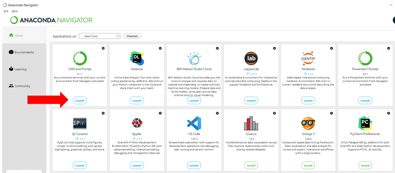
Figure 1. Launch CMD.exe Prompt

Install spaCy

spaCy is a free, open-source library for Natural Language Processing in Python with features for common tasks like tagging, parsing, Named Entity Recognition (NER), lemmatization, etc. This article will use spaCy for lemmatization, which is the process of converting words to their root. For example, the lemma of words like ‘walking’, ‘walks’ is ‘walk’. Lemmatization uses contextual vocabulary and morphological analysis to produce better outcomes than stemming. You can learn more about lemmatization and stemming here.

Run the following code in the CMD.exe Prompt, to install (or update if already installed) the spaCy package, along with its prerequisites.

 

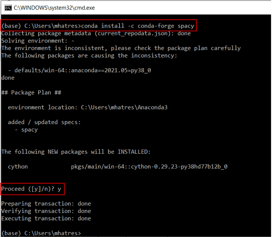
Figure 2. Install spaCy package

Run the following code in CMD.exe Prompt, to download en_core_web_sm trained pipeline for English language

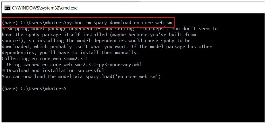
Figure 3. Download en_core_web_sm trained pipeline for English

Please refer to spaCy Installation guide for detailed instructions and troubleshooting of common issues.

Install wordcloud

The wordcloud package is used to create the word cloud visualization, where the size of each keyword indicates its relative frequency within a particular text document.

Run the following code in CMD.exe Prompt to install the wordcloud package.

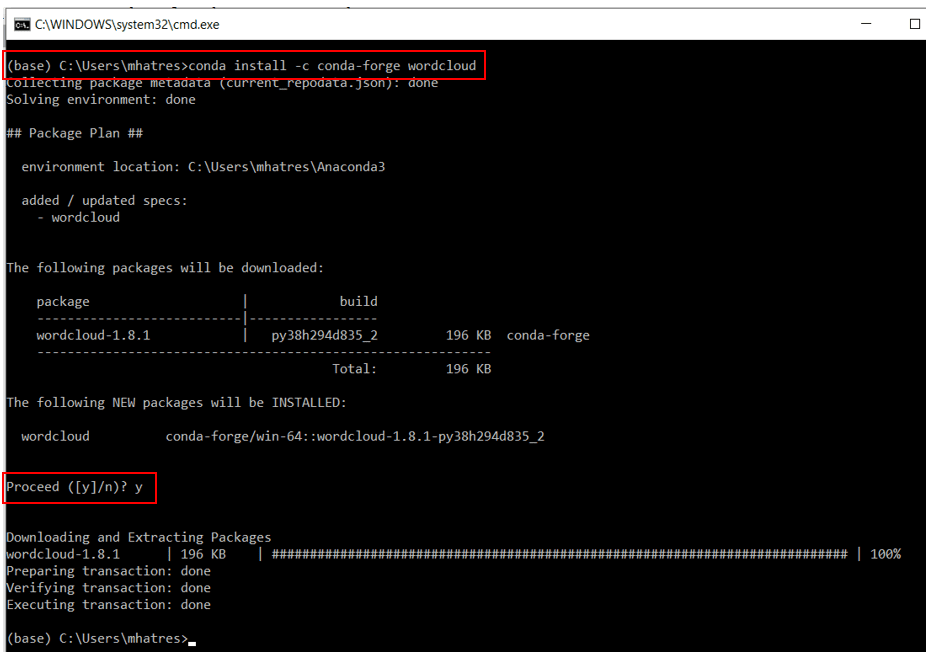
Figure 4. Install wordcloud package

Restart the Jupyter notebook Kernel so it can use the newly installed spaCy and wordcloud packages.

 

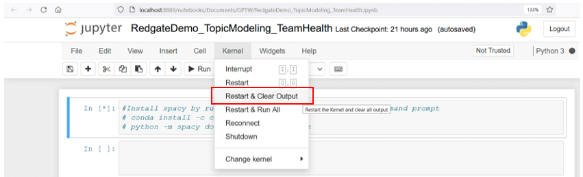
Figure 5. Restart Jupyter notebook Kernel

Install Gensim and pyLDAvis

Gensim is an open-source library for Natural Language Processing focusing on performing unsupervised topic modeling. The demo code in this article uses features specific to genism version 3.8.3 and may not work as expected with other versions of this library.

pyLDAvis is an open-source package to build interactive web-based visualizations

Run the following commands in the first cell of the Jupyter notebook to install genism and pyLDAvis

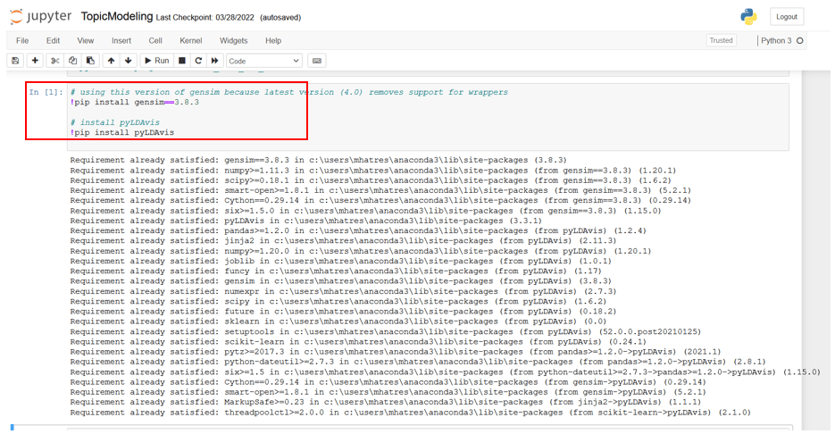
Figure 6. Install genism and pyLDAvis from Jupyter notebook

Import Natural Language Processing modules

This section introduces readers to modules used for Natural Language Processing (NLP) in this article

• re module provides operations for regular expression matching, useful for pattern and string search.
• pandas is one of the most widely used open-source tools for data manipulation and analysis. Developed in 2008, pandas provides an incredibly fast and efficient object with integrated indexing called DataFrame. It comes with tools for reading and writing data from and to files and SQL databases. It can manipulate, reshape, filter, aggregate, merge, join and pivot large datasets and is highly optimized for performance.
• NumPy is a library for Python that offers comprehensive mathematical functions that can operate upon large, multi-dimensional arrays and matrices
• pprint module in Python provides the ability to pretty-print arbitrary Python data structures that are otherwise hard to visualize
• Gensim is an open-source library for Natural Language Processing focusing on performing unsupervised topic modeling.
• spaCy is a free open-source library for Natural Language processing in Python with features for common tasks like tagging, parsing, Named Entity Recognition (NER), lemmatization, etc.
• pyLDAvis parses the output of a fitted LDA topic model into a user-friendly interactive web-based visualization. It enables data scientists to interpret the topics in a fitted topic.
• matplotlib is an easy-to-use, popular, and comprehensive library in Python for creating visualizations. It supports basic plots (like line, bar, scatter, etc.), plots of arrays & fields, statistical plots (like histogram, boxplot, violin, etc.), and plots with unstructured coordinates.
• Natural Language Toolkit, commonly known as NLTK, is a comprehensive open-source platform for building applications to process human language data. It comes with powerful text processing libraries for typical Natural Language Processing (NLP) tasks like cleaning, parsing, stemming, tagging, tokenization, classification, semantic reasoning, etc. NLTK has user-friendly interfaces to several popular corpora and lexical resources, Word2Vec, WordNet, VADER Sentiment Lexicon, etc.
• Wordcloud library is used to create the word cloud visualization

Run this code snippet in the next cell of the Jupyter notebook to load the necessary modules. Please note that this step may need a few minutes to complete.

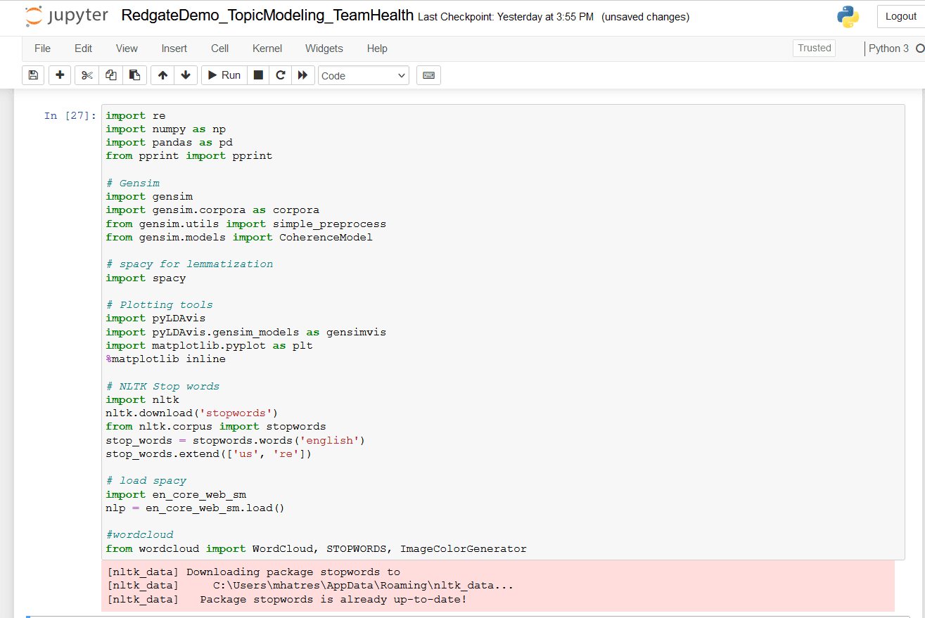
Figure 7. Load NLP modules

Load and clean demo dataset

This step uses read_excel method from pandas to load the demo input datafile into a pandas dataframe. The code below also cleans text in the Response field by

• Converting the Response field to string datatype
• Converting all text to lowercase
• Removing all non-alphabet characters

Run this code snippet in the next cell of the Jupyter notebook.

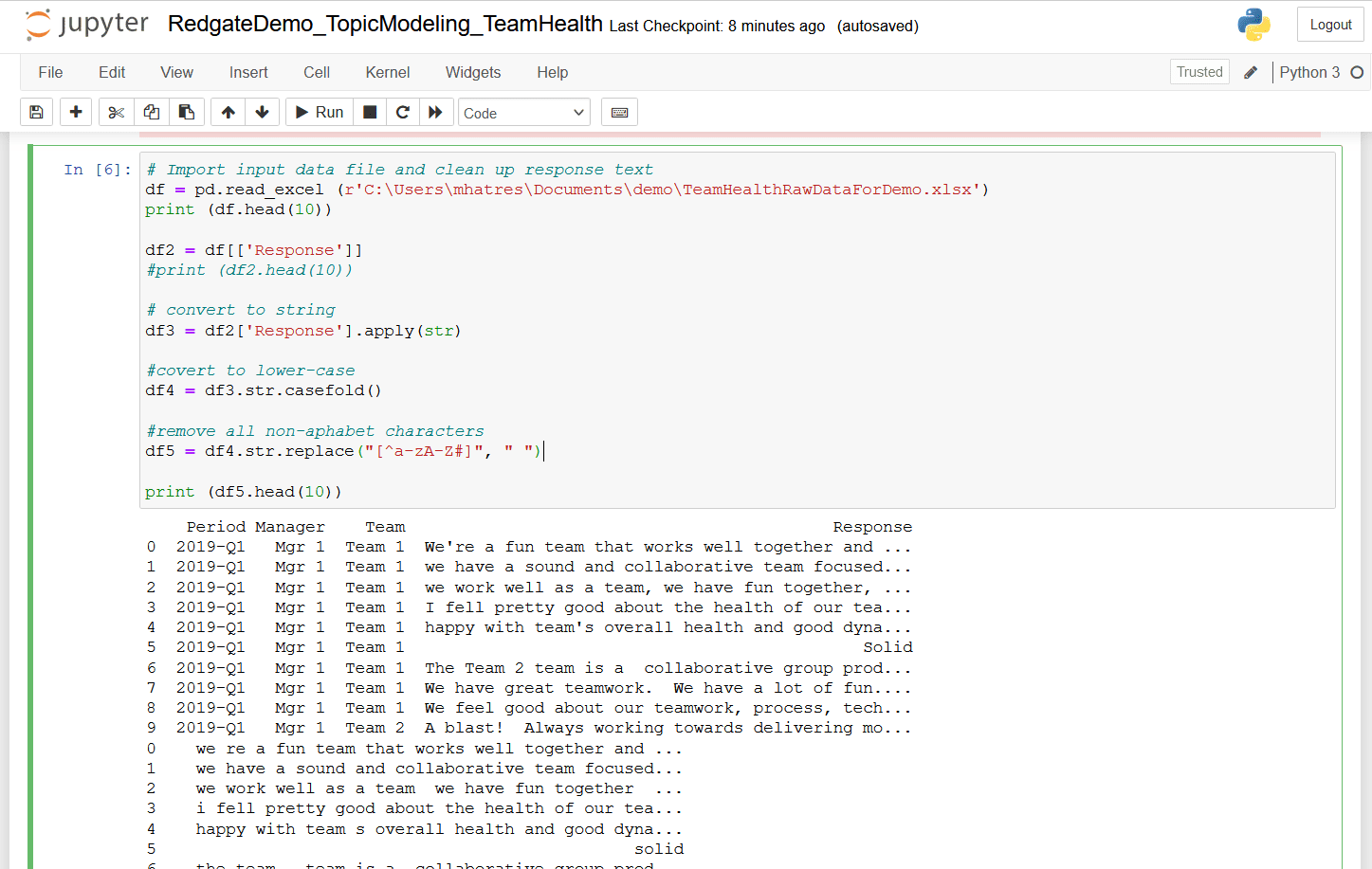
Figure 8. Load and clean demo dataset

Generate a Word Cloud

The word cloud visualization shows which keywords occur most frequently in the given text. Words with higher frequency are indicated by their larger size in the visual. Run this code snippet in the next cell of the Jupyter notebook.

 

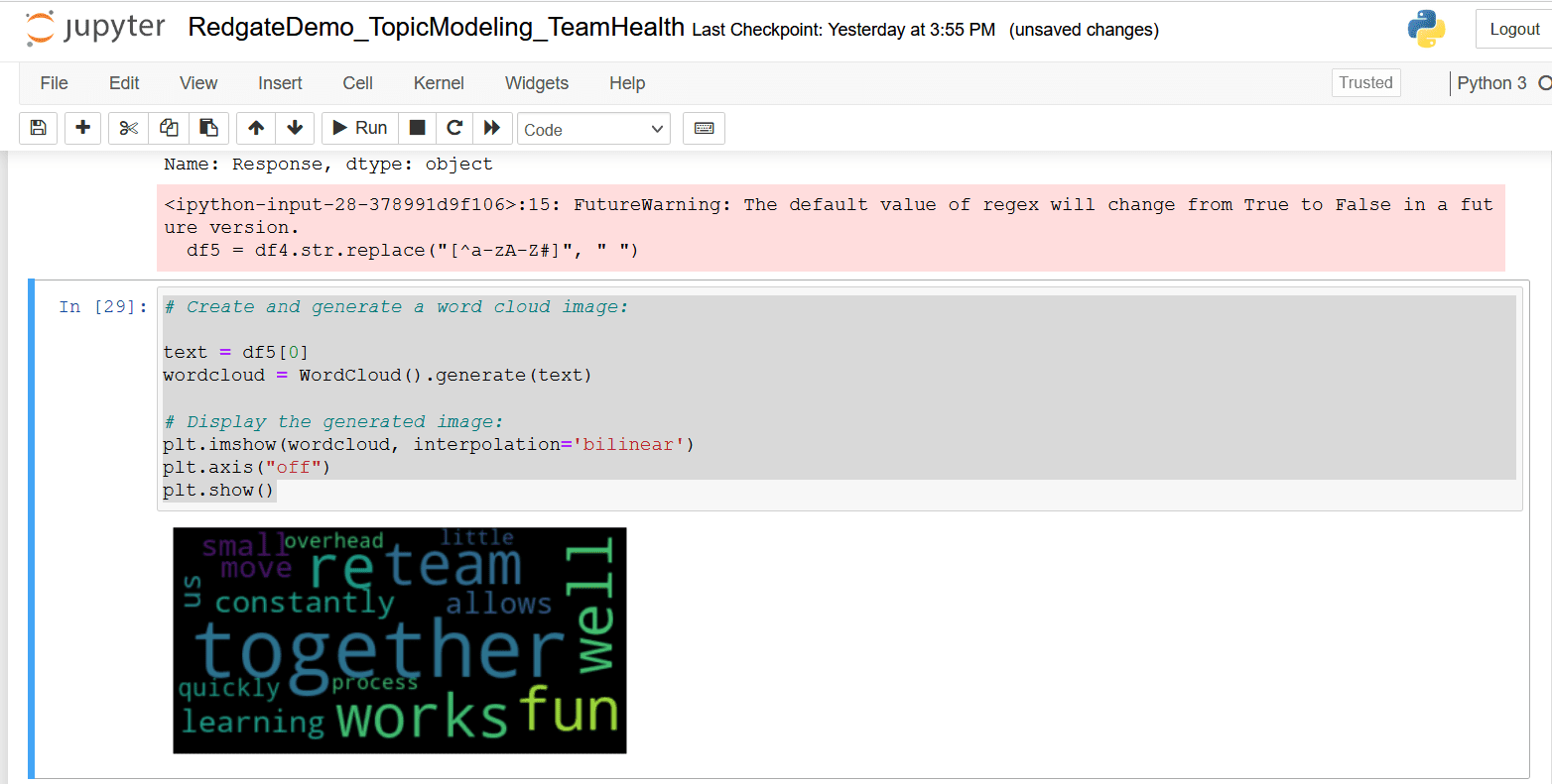
Figure 9. Word Cloud visual

This word cloud visual indicates ‘together’ is the most frequent keyword in this text, followed by ‘works,’ ‘fun,’ ‘well,’ and ‘team’. While these words have positive connotations, it’s difficult to gain deeper insights from this word cloud.

Topic Modeling

Topic modeling using LDA involves several steps and, in its most basic form, can be an iterative approach, with opportunities for further automating the process of running iterations. This section walks readers through the process of gaining deeper insights from this demo dataset using topic modeling.

Step 1: Tokenization

Tokenization in Natural Language Processing (NLP) is the process of separating a body of text into smaller units called tokens. Tokenization can be performed at ‘word,’ ‘characters,’ and ‘sub-word (n-gram character)’ levels. Tokens are considered building blocks of any natural language and popularly used NLP techniques work at the token level. Tokenization is usually a fundamental step in most Natural Language Processing projects.

A sentence or phrase composed of two words is called a bigram, and one composed of three words is called a trigram. Common examples of such phrases in this demo text include ‘fun team,’ ‘small overhead,’ and ‘constantly learning together.’

Run the following code snippet in the next cell of the Jupyter notebook to tokenize words and create bigram/trigram models.

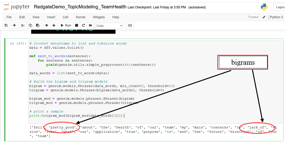
Figure 10. word tokenization, bigrams, and trigrams

You can tune the parameters of min_count and threshold and re-run this cell multiple times to arrive at a reasonable output sample. The ability of these models to identify larger quantities of bigrams/trigrams diminishes as these parameters are set to higher values, however, the quality of the ones identified can improve. The sweet spot can be identified after a few iterations.

Step 2: Stop words, n-grams, and lemmatization

Stop words are any words that should be filtered out (typically by adding to a stop list) during natural language processing. In the English language, words which don’t add much value to the sentence and can be safely ignored without compromising their meaning are typically included in a predefined stop list. Examples of stop words in English include ‘a,’ ‘the,’ ‘have,’ etc. Stop lists can be augmented with custom stop words as needed.

Run this code snippet in the next cell of the Jupyter notebook to define functions for removing stop words, creating n-grams, and performing lemmatization.

Then run this code snippet to call these functions in order.

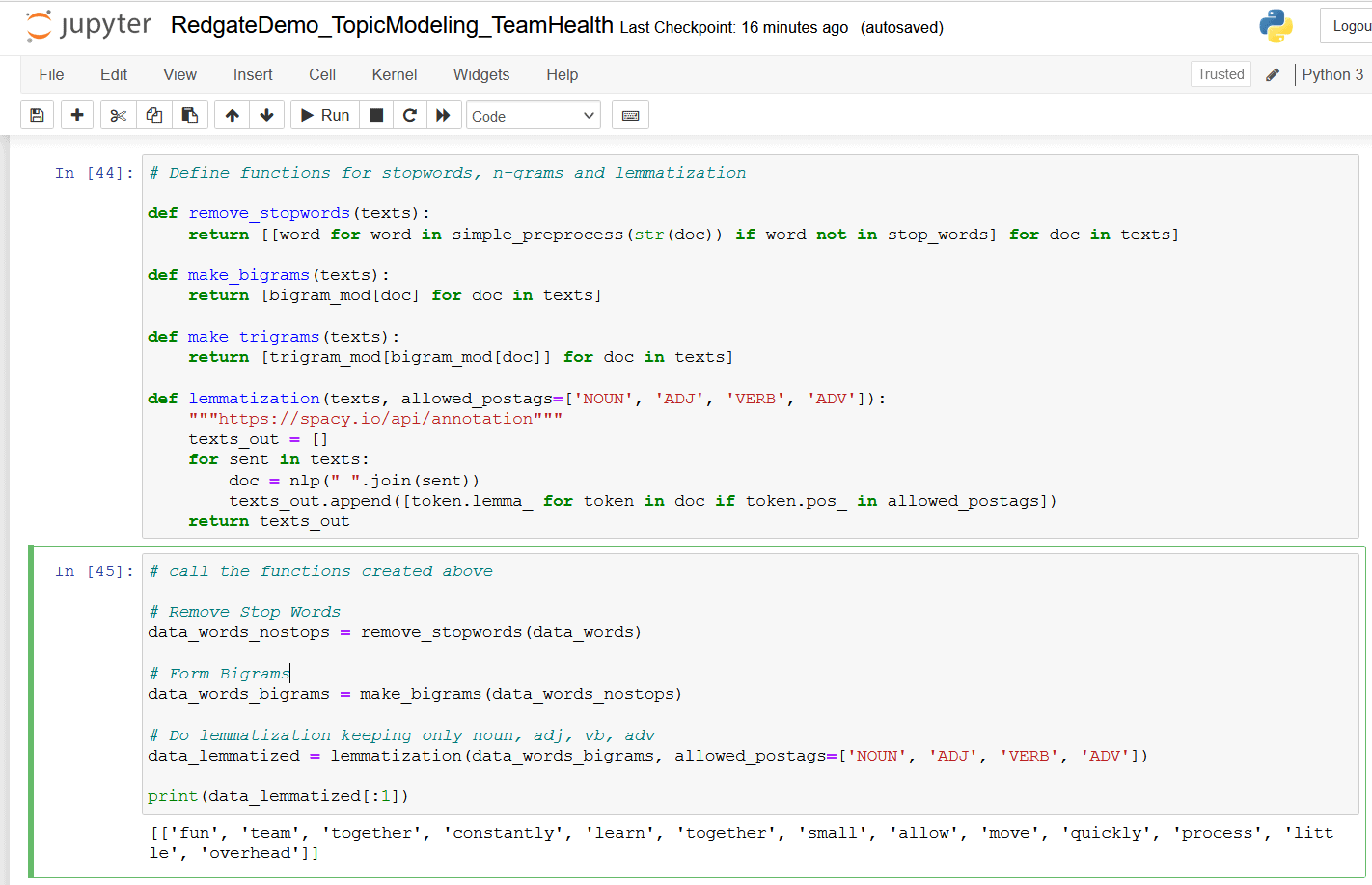
Figure 11. Stop words, n-grams, and lemmatization

Step 3: Create dictionary and corpus

The LDA topic model needs a dictionary and a corpus as inputs. The dictionary is simply a collection of the lemmatized words. A unique id is assigned to each word in the dictionary and used to map the frequency of each word and to produce a term document frequency corpus. A corpus (Latin for body) refers to a collection of texts.

Run this code snippet in the next cell of the Jupyter notebook to create the dictionary, the term document frequency corpus, and view a sample of its contents.

 

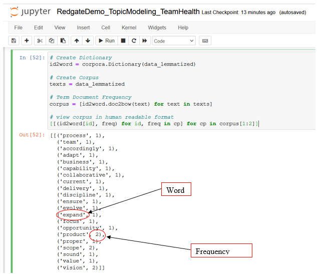
Figure 12. Dictionary and corpus of word term-frequency

Step 4: Build the LDA topic model

This section trains LDA model from the Gensim library using the models.ldamodel module.

• Corpus and id2word (dictionary) are the two key inputs parameters prepared in the previous steps
• num_topics parameter specifies the number of topics to be extracted from the input corpus. Set this value to 2 initially. I will iterate through a few values of this parameter to find the optimal topic model
• update_every parameter determines how often the model parameters should be updated as several rounds of training passes are made. Set it to 1
• chunksize parameter specifies the number of documents to be used in each training chunk. Set it to 100
• passes parameter determines the number of training passes. Set it to 10
• per_word_topic is set to True, which tells the model to compute a list of topics sorted in the descending order of most likely topics for each word
• alpha is an optional parameter related to document-topic distribution. Setting it to auto allows the model to learn an asymmetric prior from the corpus

Run this code snippet in the next cell of the Jupyter notebook to train the LDA topic model and print keywords for each topic along with their importance scores.

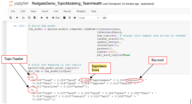
Figure 13. Train LDA topic model and infer extracted topics

• The output shows two topics (topic 0 and topic 1), along with the top ten keywords within each topic and their importance scores
• The keywords of topic 0 seem to indicate ‘good overall team health’
• The keywords of topic 1 seem to indicate ‘great work, feel good support (in) team, lot (of) fun’
• This manual interpretation of topics is commonly known as ‘labeling’ or ‘tagging’ of extracted topics

Since this is an unsupervised learning technique, it remains unclear if two is the right number of topics present in this text. The subsequent steps will help answer the question: “Does this text document have any more useful topics to extract?”

Step 5: Compute model performance metrics

Model perplexity and topic coherence are useful metrics to evaluate the performance of a trained topic model.

The model perplexity measures how perplexed or surprised a model is when it encounters new data. Measured as a normalized log-likelihood of a held-out test set, it’s an intrinsic metric widely used for language model evaluation. While a perplexity value closer to zero indicates a better model, optimizing for perplexity may not always lead to human readable topics.

Topic Coherence measures the degree of semantic similarity between high-scoring words within the same topic. A set of words, phrases, or statements can be defined as ‘coherent’ if they support each other. This metric can help to differentiate between human interpretable semantic topics versus topics that are outcomes of statistical inference but have very little semantic value.

Run this code snippet in the next cell of the Jupyter notebook to generate model perplexity and coherence score.

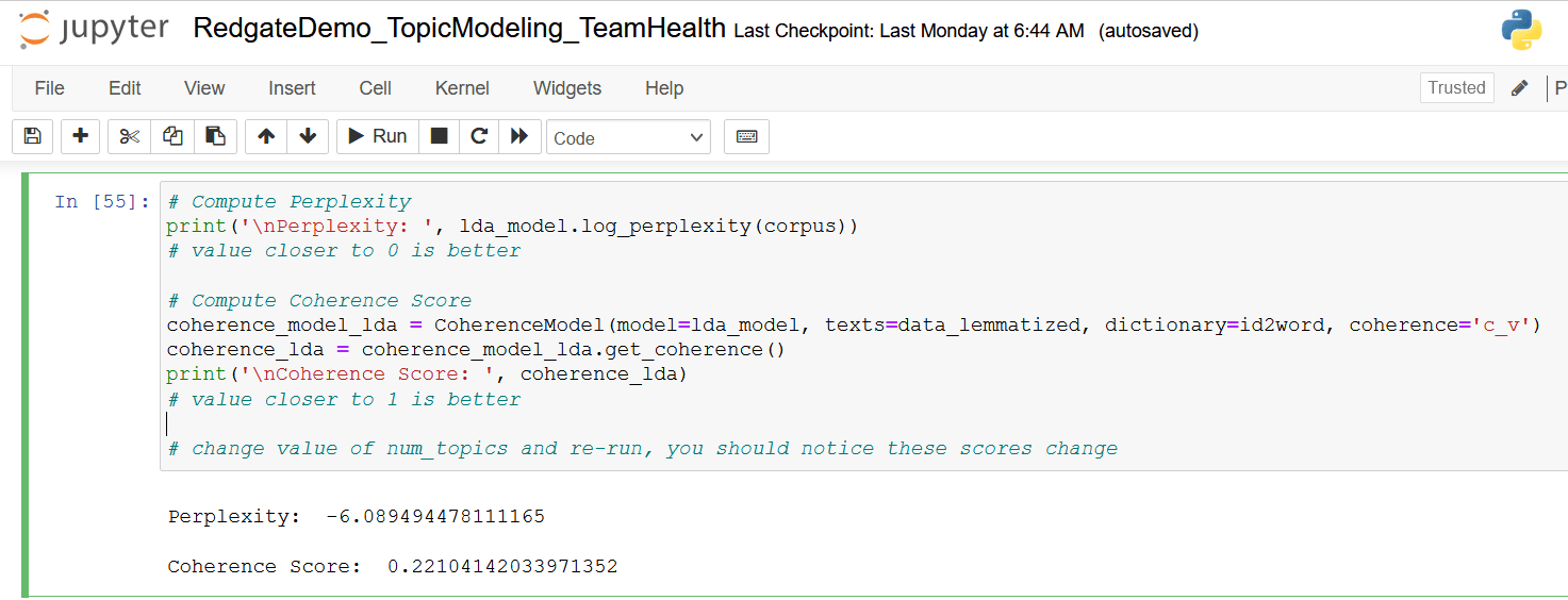
Figure 14. Perplexity and Coherence scores

Make a note of Perplexity and Coherence scores in Figure 14, as you will retrain the model with updated values for the num_topic parameter and recompute these metrics.

Step 6: Visualization

The pyLDAvis package is a great tool to generate an interactive chart to visualize the inter-topic distance map and examine the keywords for each topic. Run this code snippet in the next cell of the Jupyter notebook to create this chart

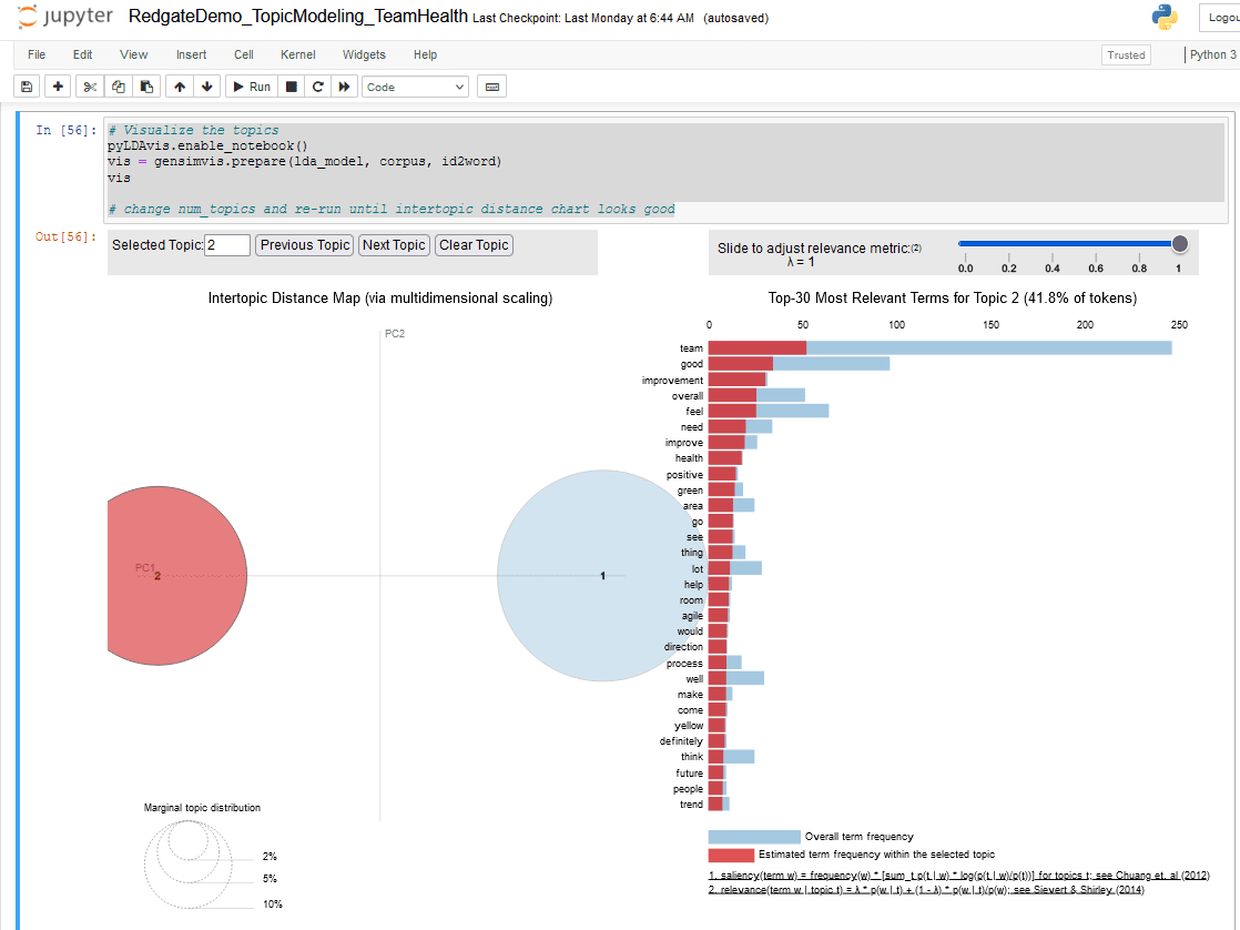
Figure 15. pyLDAvis chart of modeled topics

• The Intertopic Distance Map on the left half of this chart represents each topic as a bubble, whose size correlates to the prevalence of its topic within the text document. An optimal topic model is represented by large, non-overlapping bubbles that are scattered throughout the chart.

A poor topic model has many small bubbles that are overlapping and/or clustered in one region of the chart. You can retrain the model by incrementing num_topics and recreating this visual, as well as use the model performance metrics to find the optimal number of topics.

• The Relevant terms per topic on the right half of this chart shows the top 30 terms (words) per topic, along with the percentage prevalence of chosen topic. It’s an interactive stacked bar chart where each blue bar represents the overall frequency of a term (word) within the document. When you select a topic by clicking on one of the bubbles on the left side, the overlapping red bars appear on the right side, indicating estimated frequency of each term within that topic.
• While your output may look different, please make a note of the top ten words for each topic.

Step 7: Retrain topic model iteratively

This step is an iterative process involving:

• Incrementing the value of num_topics parameter and rebuild the LDA topic model (step 4)
• Noting values of model performance metrics (step 5)
• Generating pyLDAvis chart and studying the Intertopic Distance Map (Step 6)
• Repeating the above three steps until the Intertopic Distance Map looks optimal

Run this code snippet in the next cell of the jupyter notebook

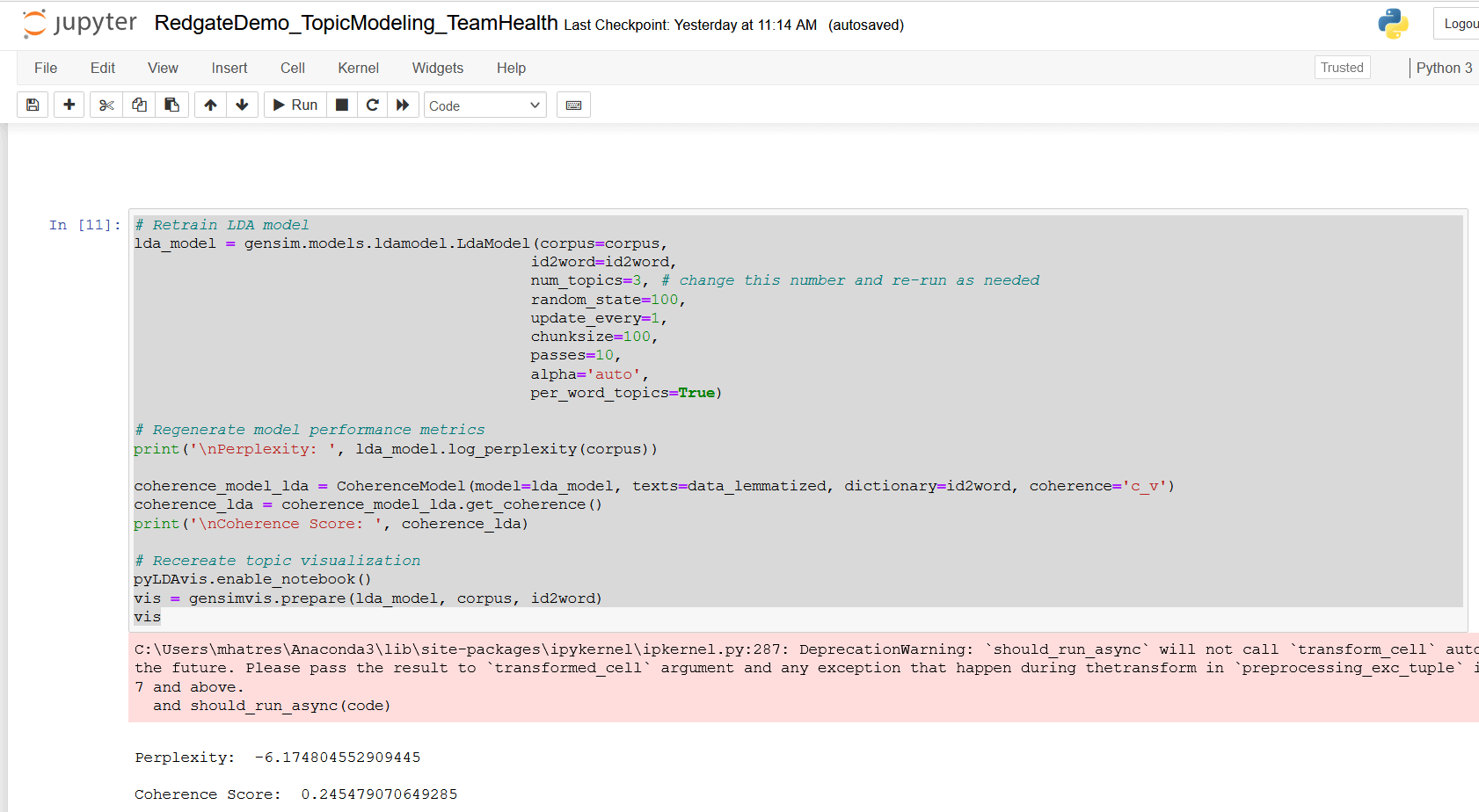
Figure 16. Retrain LDA topic model with num_topics = 3

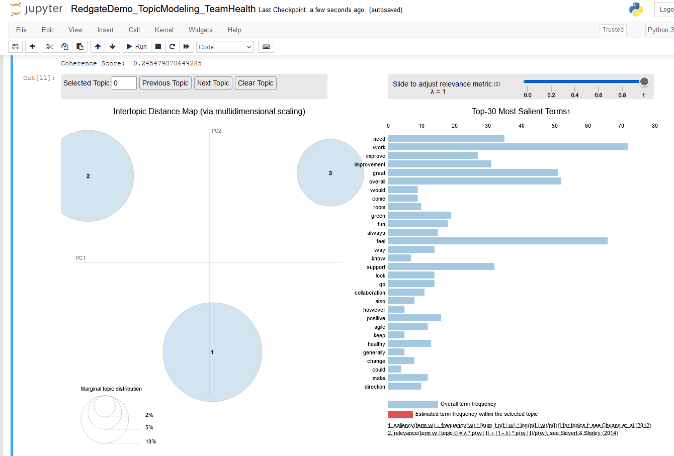
Figure 17. pyLDAvis chart for three topics

Repeat the above steps by setting value of num_topics parameter to four (4).

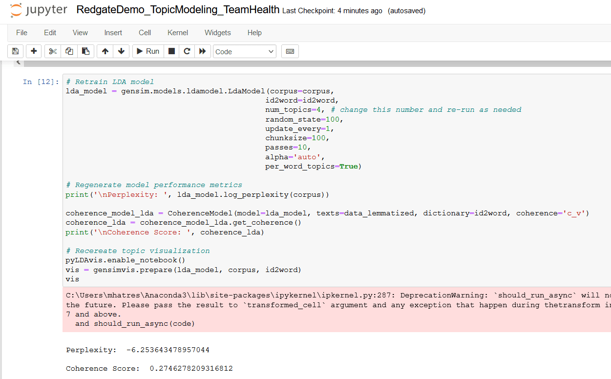
Figure 18. Retrain LDA topic model with num_topics = 4

Overlapping bubbles indicate a poor model

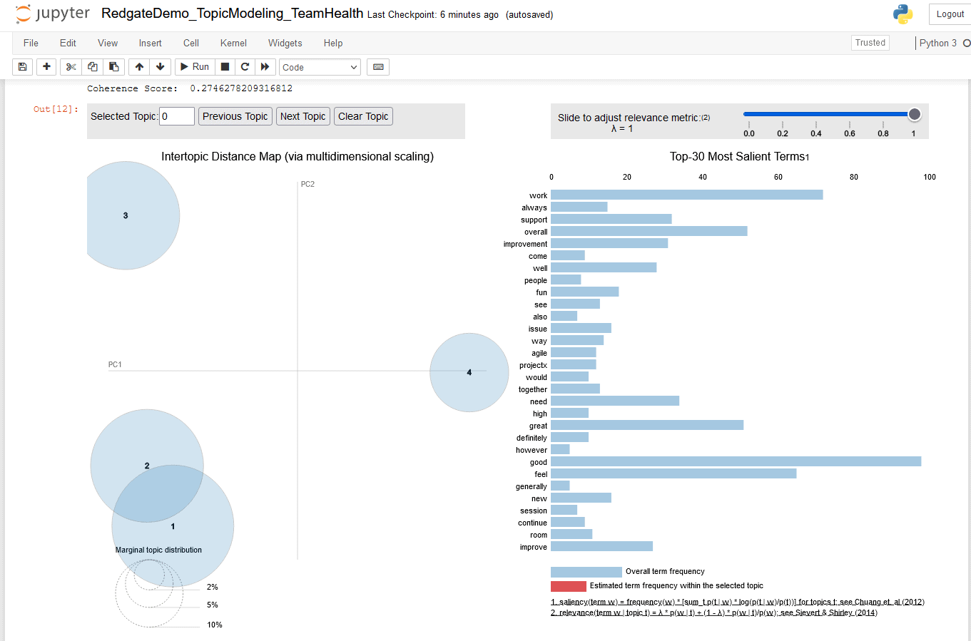
Figure 19. pyLDAvis chart for four topics

The Intertopic Distance Map shows bubbles for topic number 1 and 3 are overlapping, which indicates I have overshot the optimal number of topics. At this point I can stop running iterations and analyze their outputs.

Num_topics	Model perplexity	Topic Coherence	Intertopic Distance Map
2	-6.089	0.221	Two large bubbles well-spaced across chart quadrants
3	-6.174	0.245	Three large bubbles well-spaced across chart quadrants
4	-6.253	0.274	Three large bubbles and one small. Bubbles for topics 1 and 2 are overlapping

Figure 20. Table of observations for three iterations

Model perplexity and Topic Coherence metrics seem to indicate model performs better as the value of num_topics parameter increases. However, the Intertopic Distance Map is optimal when num_topics parameter is set to 3. These factors lead me to conclude that three topics is the optimal number of topics I can extract from this text document.

Your Intertopic Distance Map might not show overlapping bubbles for num_topics = 4, and you may need to continue running more iterations by incrementing num_topics until your Intertopic Distance Map shows overlapping bubbles. In this case, it’s helpful to make a note of the top ten keywords for each topic in each iteration, so you can identify if keywords are repeating between different topics within the same iteration.

Step 8. Infer topic labels

After identifying the optimal number of topics, the next step is to infer human-readable labels for each topic using their frequent terms. This step is not an exact science and typically benefits from a good understanding of the business context of your dataset.

Revisit the pyLDAvis chart for iteration where num_topics is set to 3, then click on bubble 1.

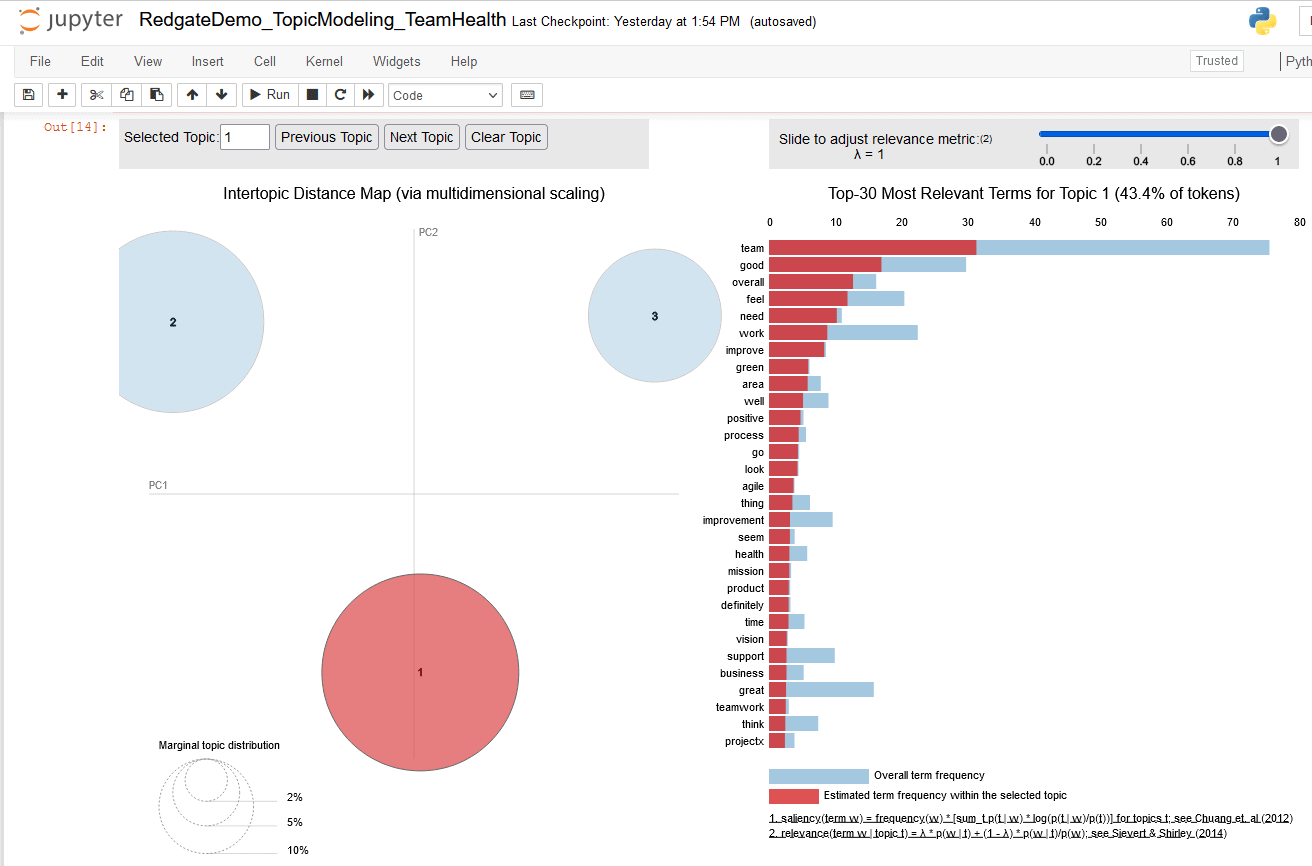
Figure 21. three topic pyLDAvis chart, highlighting terms for topic 1

This figure focuses on bubble for topic 1 and indicates

• Topic 1 includes 43.4 % of tokens found in the text document
• The top 10 terms of topic 1 are used to infer label ‘Overall Team (health) feel(s) good, positive (and) green’ (I have used business context knowledge of the Team Health survey process to associate ‘green’ with good team health).

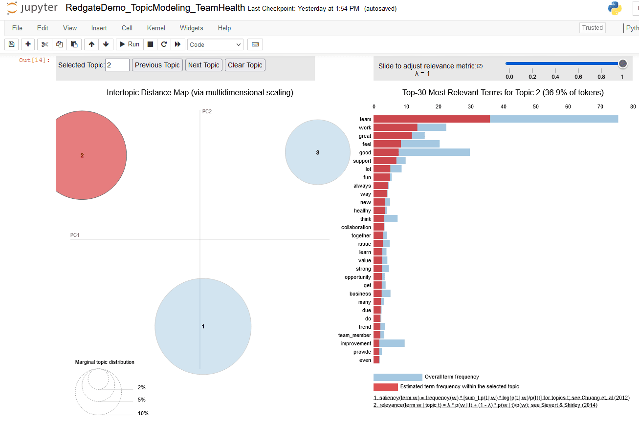
Figure 22. Three topic pyLDAvis chart, highlighting terms for topic 2

This figure focuses on bubbles for topic 2 and indicates:

• Topic 2 includes 36.9 % of tokens found in the text document
• The top 10 terms of topic 2 are used to infer label ‘Great work, good support (and) lot (of) fun’

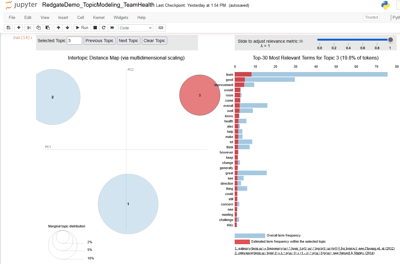
Figure 23. Three topic pyLDAvis chart, highlighting terms for topic 1

This figure focuses on bubble for topic 3 and indicates:

• Topic 3 includes 19.8 % of tokens found in the text document
• The top 10 terms of topic 3 are used to infer label ‘Room (for) improvement’

If your Intertopic Distance Map does not show overlapping bubbles for num_topics = 4, you may need to continue running more iterations by incrementing num_topics until your Intertopic Distance Map shows overlapping bubbles. Please make note of the top ten keywords for each topic in each iteration. This is helpful to detect when keywords are repeating between different topics within the same iteration, even if the Intertopic Distance Map looks great, which indicates you have overshot the optimal number of topics.

Automation

This use case is simple and needs only three iterations to arrive at an optimal solution. A very complex use case may need several tens of iterations to find the optimal topic model. Running so many iterations manually can become a tedious chore. There are a few options to automate the process of running iterations

• Program a Loop
  • Write a loop to iterate the num_topics from 2 to 30 (or any upper value of your choice based on your business context knowledge of the data set).
  • Plot model performance metrics as a line chart against num_topics on, to identify the value of num_topics where these metrics stop improving
  • Save the pyLDAvis chart for each iteration in a folder and review the Intertopic Distance Maps to find the optimal number of human readable topics
• LDA Mallet Model
  • Mallet is an open-source toolkit for NLP with a package for LDA based topic modeling
  • Gensim provides a wrapper to facilitate Mallet’s LDA topic model estimation and inference of topic distribution
  • It handles running iterations without having to code a loop

Exploring these automation options in detail is outside the scope of this article

Compare Topic modeling and Word Cloud

The process of topic modeling with LDA helped discover deeper insights from the Team Health survey responses in the form of following three topics:

Topic Number	Percentage Composition of Tokens	Topic Label
1	43.3 %	Overall Team health is good/positive
2	36.9 %	Great work, lot of fun and supportive team
3	19.8 %	Some room for improvement

Figure 24. Summary of Insights from Topic modeling

These topics help to deliver actionable analysis to business stakeholders. Combined with business context, subject matter expertise, and organizational knowledge, the following might be a good a summary readout to potential business stakeholder group of IT leadership.

• The prevalent consensus (43.3 %) amongst survey respondents indicates that overall Team health is good/positive
• Over a third (36.9 %) of survey responses indicate teams are supportive of their members, they have lot of fun, and work is great (positive environment for teamwork)
• Around one fifth (19.8 %) of survey responses hint at some room for improvement

Comparing these richer insights against the Word Cloud from Figure 9, highlights the Word Cloud’s shortcomings and helps readers gain an appreciation for the deeper insights uncovered by Topic Modeling.

Deeper Insights with Topic Modeling

This article walked readers through the process of Topic modeling with LDA and understanding the value of its deeper insights, especially when compared to easier techniques like Word Cloud. Through the course of this article, I demonstrated:

• Setup of Anaconda Jupyter notebook environment for performing topic modeling
• Data cleaning and preparation steps needed for topic modeling with LDA
• Iterative process of training topic models and identifying an optimal solution
• Interpreting human readable insights from topic model output charts
• Comparing these deeper insights with outcomes from the easier technique of word cloud
• Business value of topic modeling as a popular and practical Natural Language processing technique

References

• Topic modeling – https://en.wikipedia.org/wiki/Topic_model
• Latent Dirichlet allocation – https://en.wikipedia.org/wiki/Latent_Dirichlet_allocation
• LDA paper from Journal of Machine Learning Research – https://www.jmlr.org/papers/volume3/blei03a/blei03a.pdf
• TF-IDF – https://en.wikipedia.org/wiki/Tf%E2%80%93idf
• Lemmatization and stemming – https://nlp.stanford.edu/IR-book/html/htmledition/stemming-and-lemmatization-1.html
• spaCy – https://spacy.io/
• tokenization – https://aclanthology.org/C92-4173.pdf
• n-grams – https://en.wikipedia.org/wiki/N-gram
• Evaluate topic models using perplexity and coherence scores – https://towardsdatascience.com/evaluate-topic-model-in-python-latent-dirichlet-allocation-lda-7d57484bb5d0
• pyLDAvis – https://pyldavis.readthedocs.io/en/latest/readme.html
• Link to the Topic modeling jupyter notebook with code and results on my Github repository – https://github.com/SQLSuperGuru/SentimentAnalysis/blob/main/TopicModeling.ipynb