The series so far:
- SQL Server R Services: The Basics
- SQL Server R Services: Digging into the R Language
- SQL Server R Services: Working with ggplot2 Statistical Graphics
- SQL Server R Services: Working with Data Frames
- SQL Server R Services: Generating Sparklines and Other Types of Spark Graphs
- SQL Server R Services: Working with Multiple Data Sets
Throughout this series, we’ve looked at several examples of how to use SQL Server R Services to create R scripts that incorporate SQL Server data. The key to using SQL Server data is to pass in a T-SQL query as an argument when calling the sp_execute_external_script stored procedure. The R script can then incorporate the data returned by the query, while taking advantage of the many elements available to the R language for analyzing data.
Despite the ease with which you can run an R script, the sp_execute_external_script stored procedure has an important limitation. You can specify only one T-SQL query when calling the procedure. Of course, you can create a query that joins multiple tables, but this approach might not always work in your circumstances or might not be appropriate for the analytics you’re trying to perform. Fortunately, you can retrieve additional data directly within the R script.
In this article, we look at how to import data from a SQL Server table and from a .csv file. We also cover how to save data to a .csv file as well as insert that data into a SQL Server table. Being able to incorporate additional data sets or save data in different formats provides us with a great deal of flexibility when working with R Services and allows us to take even greater advantage of the many elements available to the R language for data analytics.
Importing data from SQL Server
When you call the sp_execute_external_script stored procedure, you can pass in a single T-SQL query to the @input_data_1 parameter. This allows you to incorporate the data returned by the query directly within your R script. In some cases, however, you might want to bring in additional data, either from SQL Server or from another source.
For example, the following T-SQL code includes an R script that retrieves data separately from the SalesOrderHeader and SalesTerritory tables in the AdventureWorks2014 database:
|
1 2 3 4 5 6 7 8 9 10 11 12 13 14 15 16 17 18 19 20 21 22 23 24 25 26 27 28 29 30 31 |
USE AdventureWorks2014; G DECLARE @rscript NVARCHAR(MAX); SET @rscript = N' # retrieve sales data from InputDataSet sales <- InputDataSet # retrieve territory data from SalesTerritory table conn <- "Driver=SQL Server; Server=localhost\\sqlsrv16b; Database=AdventureWorks2014; Uid=user1; Pwd=password1" query <- "SELECT TerritoryID, Name FROM Sales.SalesTerritory;" territories <- RxSqlServerData(connectionString = conn, sqlQuery = query) territories <- rxDataStep(territories) # merge data sets based on territory IDs df1 <- merge(territories, sales, by = "TerritoryID") names(df1) <- c("TerritoryID", "Territory", "Sales") # build data frame with aggregated data c1 <- levels(as.factor(df1$Territory)) c2 <- round(tapply(df1$Sales, df1$Territory, mean)) df2 <- data.frame(c1, c2) OutputDataSet <- df2'; DECLARE @sqlscript NVARCHAR(MAX); SET @sqlscript = N' SELECT TerritoryID, Subtotal FROM Sales.SalesOrderHeader;'; EXEC sp_execute_external_script @language = N'R', @script = @rscript, @input_data_1 = @sqlscript; GO |
If you reviewed the previous articles in the series, you should be familiar with how to call the sp_execute_external_script stored procedure and run an R script. In this article, we focus primarily on the components within the R script. If you’re uncertain about the other language elements, be sure to refer to the previous articles.
The first element in the R script assigns the data retrieved from the SalesOrderHeader table to the sales variable, using the InputDataSet variable to access the SQL Server data:
|
1 |
sales <- InputDataSet |
This gives us our first data set, which includes the sale amounts associated with the individual territory IDs. Now suppose we want to use territory names rather than IDs. We can do this in our original T-SQL query by joining the two tables, or we can call the tables individually. In this case, the tables are in the same database, so creating one query would be the most expedient approach, but data is not always accessible through a join, or sometimes an R script requires a different approach to working the data, such as needing to join data after aggregating one of the data sets.
For this example, our primary purpose is to demonstrate how to bring in a second data set from SQL Server, so we’ll retrieve the territory data separately. To do so, we must first define a connection to the SQL Server instance that contains the data:
|
1 2 3 4 5 |
conn <- "Driver=SQL Server; Server=localhost\\sqlsrv16b; Database=AdventureWorks2014; Uid=user1; Pwd=password1" |
To define the connection, we create a single string that specifies the driver, instance, database, user ID, and password, separated by semi-colons. Note that you should not put spaces around the equal signs within the connection definition. If you do, you will receive an error.
You can also define a connection that uses Windows Authentication, rather than having to provide a user name and password. If you take this approach, your connection definition would look similar to the following:
|
1 2 3 4 |
conn <- "Driver=SQL Server; Server=localhost\\sqlsrv16b; Database=AdventureWorks2014; Trusted_Connection=True" |
To use Windows Authentication, you might have to set up implied authentication on the target SQL Server instance, as described in the Microsoft article Modify the User Account Pool for SQL Server R Services.
After we set up the connection, we can define a SELECT statement to retrieve the data we need from the SalesTerritory table:
|
1 |
query <- "SELECT TerritoryID, Name FROM Sales.SalesTerritory;" |
With our connection and query in place, we can use the RxSqlServerData function to generate a SQL Server data source object:
|
1 |
territories <- RxSqlServerData(connectionString = conn, sqlQuery = query) |
The RxSqlServerData function is part of the RevoScaleR library included with R Services. The library includes a collection of functions for importing, transforming, and analyzing data at scale. A subset of those functions, including RxSqlServerData, is specific to SQL Server.
Using the RxSqlServerData function in this way gives us our second data set, which we assign it to the territories variable.
Another SQL Server function in the RevoScaleR library is rxDataStep. We can use the function in an R script to transform the data returned by the RxSqlServerData function into a more workable format. Our next step, then, is to run the function against the territories data set, assigning the results back to the same variable:
|
1 |
territories <- rxDataStep(territories) |
Not surprisingly, there’s a lot more to the RevoScaleR library and SQL Server functions than what we’ve covered here, so be sure to check out the rest when you have time. A good place to start is with the Microsoft topic RevoScaleR package.
With our two data sets in place, we can use the merge function to create a single data frame, joining the data sets based on the TerritoryID column in each one:
|
1 |
df1 <- merge(territories, sales, by = "TerritoryID") |
We can then use the names function to assign names to the data frame columns, making it easier to work with the data frame later in the script:
|
1 |
names(df1) <- c("TerritoryID", "Territory", "Sales") |
We now have a single data frame, df1, that contains the data we need to move forward with our (simple) analytics. The next step is to create a second data frame that aggregates the data based on the sales amounts. The goal is to come up with the mean sales per territory. To do this, we construct the new data frame one column at a time, starting with a column that lists the individual territory names:
|
1 |
c1 <- levels(as.factor(df1$Territory)) |
We begin by using the as.factor function to convert the values in the Territory column to a factor, which provides a way for us to work with categorical data. We can then use the levels function to retrieve the distinct territory names, assigning them to the c1 variable.
The next step is to define the column that will contain the aggregated sales data:
|
1 |
c2 <- round(tapply(df1$Sales, df1$Territory, mean)) |
We start by using the tapply function to aggregate the sales totals for each category. The first argument, df1$Sales, indicates that the Sales values are the ones to be aggregated. The second argument, df1$Territory, provides the basis for the aggregation, in this case, the territories. The territory names also serve as an index for the c2 column. The third argument, mean, indicates that the mean sales value should be calculated for each territory. We then use the round function to round the aggregated totals to integers.
With our two column definitions in place, we can use the data.frame function to create a data frame and assign it to the df2 variable:
|
1 |
df2 <- data.frame(c1, c2) |
At this point, we can take any number of other steps as part of our analytics, but we’ll stop here. The only remaining task is to assign the df2 data frame to the OutputDataSet variable:
|
1 |
OutputDataSet <- df2 |
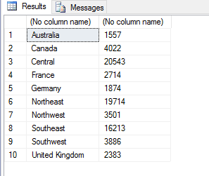
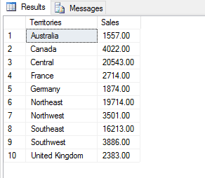
Assigning the data frame to the OutputDataSet variable makes it possible for the R script to return the data to the calling application (in this case, SQL Server Management Studio). The following figure shows the results returned by the script when we run the sp_execute_external_script stored procedure.
That’s all there is to incorporating additional SQL Server data into an R script, when a single T-SQL query not be enough. Although this is only a very basic example, it points to the potential for creating far more complex analytics that can include whatever data is necessary, as long as the target SQL Server instance is accessible from the instance running the script.
Adding conditional logic to an R script
Before we move on to importing data from a .csv file, I want to demonstrate another SQL Server function in the RevoScaleR library: rxSqlServerTableExists. The function checks whether a specified SQL Server table exists, information we can use in our R script to implement conditional logic. For example, the following script uses the function to verify whether the SalesTerritory table exists before trying to retrieve data from that table:
|
1 2 3 4 5 6 7 8 9 10 11 12 13 14 15 16 17 18 19 20 21 22 23 24 25 26 27 28 29 30 31 |
DECLARE @rscript NVARCHAR(MAX); SET @rscript = N' # retrieve sales data from InputDataSet sales <- InputDataSet # define connection to SQL Server conn <- "Driver=SQL Server; Server=localhost\\sqlsrv16b; Database=AdventureWorks2014; Uid=user1; Pwd=password1" # define conditional logic table = "Sales.SalesTerritory" if (rxSqlServerTableExists(table, connectionString = conn)) { # retrieve territory data from SalesTerritory table query <- "SELECT TerritoryID, Name FROM Sales.SalesTerritory;" territories <- RxSqlServerData(connectionString = conn, sqlQuery = query) territories <- rxDataStep(territories) # merge data sets based on territory IDs df1 <- merge(territories, sales, by = "TerritoryID") names(df1) <- c("TerritoryID", "Territory", "Sales") # build data frame with aggregated data c1 <- levels(as.factor(df1$Territory)) c2 <- round(tapply(df1$Sales, df1$Territory, mean)) df2 <- data.frame(c1, c2) } else { # build data frame with aggregated data c1 <- levels(as.factor(sales$TerritoryID)) c2 <- round(tapply(sales$Subtotal, sales$TerritoryID, mean)) df2 <- data.frame(c1, c2) } OutputDataSet <- df2'; |
Most of the script elements should look familiar, but notice that after setting up the connection, we create an if…else structure to define the conditional logic, starting with the following statements:
|
1 2 |
table = "SalesTerritory" if (rxSqlServerTableExists(table, connectionString = conn)) |
We begin by identifying the target table and assigning it to the table variable. We then use the rxSqlServerTableExists function to check if the table exists. If it does, the function returns TRUE, and the if block runs, creating the df2 data frame, just like in the preceding example.
If the function returns FALSE, the else block runs instead, creating the data frame based on territory IDs, rather than names.
In this case, we’re using the rxSqlServerTableExists function to implement conditional logic; however, you might also find it useful for verifying a table’s existence before trying to delete it or performing other operations in the R script.
However, even if you don’t use the function, the example points to something more important: the ability to implement conditional logic within R scripts, making it possible to work with SQL Server data in ways that can get quite difficult with T-SQL alone, especially when trying to perform sophisticated analytics.
Importing data from a .csv file
Rather than bringing additional data in from SQL Server, we might want to create an R script that uses data from another source, in addition to the data provided by the primary T-SQL query. For example, suppose the territory names we retrieved in the preceding examples are in a .csv file, as shown in the following figure.
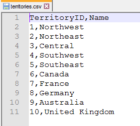
This is the same data we had retrieved from the SalesTerritory table in the preceding examples. We can update that script to instead point to that file:
|
1 2 3 4 5 6 7 8 9 10 11 12 13 14 15 |
DECLARE @rscript NVARCHAR(MAX); SET @rscript = N' # retrieve sales data from InputDataSet sales <- InputDataSet # retrieve territory data from territories.csv file inputcsv <- "C:\\DataFiles\\territories.csv" territories <- read.csv(file = inputcsv, header = TRUE, sep = ",") # merge data sets based on territory IDs df1 <- merge(territories, sales, by = "TerritoryID") names(df1) <- c("TerritoryID", "Territory", "Sales") # build data frame with aggregated data c1 <- levels(as.factor(df1$Territory)) c2 <- round(tapply(df1$Sales, df1$Territory, mean)) df2 <- data.frame(c1, c2) OutputDataSet <- df2'; |
Rather than defining a connection like we do for SQL Server, we can read the data directly from the .csv file. To do so, we first specify the file location and save it to the inputcsv variable:
|
1 |
inputcsv <- "C:\\DataFiles\\territories.csv" |
Note the use of the double backslashes to escape the single backslash. We can then use the read.csv function to retrieve the data, passing in the inputcsv variable for the file argument:
|
1 |
territories <- read.csv(file = inputcsv, header = TRUE, sep = ",") |
In addition to setting the file argument, we set the header argument to TRUE because the column names are included in the file, and we specify a comma (within quotes) for the sep argument, which indicates that a comma is used to separate the values within the file. That’s all there is to it. We can then create the df1 and df2 data frames just like we did in the preceding examples. The R script will return the same results as before.
Being able to import data from a .csv file can be useful whenever we need data other than what is available in SQL Server. This approach also allows us to get data from a legacy system, in which direct access is not possible.
And we’re not limited to .csv files. The R language lets us import data from a wide range of sources, including JSON and XML files, relational databases, non-relational data stores, web-based resources, and many more. That said, I have not tested all these source types from within R Services. The only way to know for sure what you can or cannot do in your particular circumstances is to try it out yourself.
Exporting data to a .csv file
There might be times when you want to export the results of your R script to a file, rather than (or in addition to) returning the data to the calling application. To send the data to a .csv file, for example, we can use the write.csv function, as shown in the following example:
|
1 2 3 4 5 6 7 8 9 10 11 12 13 14 15 16 17 |
DECLARE @rscript NVARCHAR(MAX); SET @rscript = N' # retrieve sales data from InputDataSet sales <- InputDataSet # retrieve territory data from territories.csv file inputcsv <- "C:\\DataFiles\\territories.csv" territories <- read.csv(file = inputcsv, header = TRUE, sep = ",") # merge data sets based on territory IDs df1 <- merge(territories, sales, by = "TerritoryID") names(df1) <- c("TerritoryID", "Territory", "Sales") # build data frame with aggregated data c1 <- levels(as.factor(df1$Territory)) c2 <- round(tapply(df1$Sales, df1$Territory, mean)) df2 <- data.frame(c1, c2) # output data to territorysales.csv file outputcsv <- "C:\\DataFiles\\territorysales.csv" write.csv(df2, file = outputcsv)'; |
Sending data to a .csv file is just as easy as retrieving it. In this case, we specify the path and target file (territorysales.csv), assigning them to the outputcsv parameter. We then use the write.csv function to write the data in the df2 data frame to the file. The following figure shows the file with the inserted data.
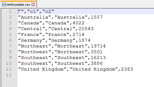
Notice that the first row includes an empty string to represent the first column and that each subsequent row includes two instances of the territory name. In this case, the R engine is also outputting the names used to index the c2 column. Plus, quotes are used to enclose the character data, which we might not want to include. We can get around these issues by modifying the write.csv function call:
|
1 |
write.csv(df2, file = outputcsv, quote = FALSE, row.names = FALSE) |
This time, when calling the function, we add two arguments. The first is quote, which we set to FALSE to specify that character data should not be enclosed in quotation marks. (You can omit this argument or set it to TRUE if you want to include the quotes.)
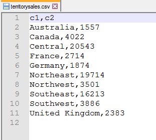
The second argument is row.names, which we set to FALSE so the extra territory names are not included, giving us the results shown in the following figure.
It should also be noted that we don’t have to choose between sending data to a file or using the OutputDataSet variable to return data to the calling application. We can do both:
|
1 2 3 4 5 6 7 8 9 10 11 12 13 14 15 16 17 18 |
DECLARE @rscript NVARCHAR(MAX); SET @rscript = N' # retrieve sales data from InputDataSet sales <- InputDataSet # retrieve territory data from territories.csv file inputcsv <- "C:\\DataFiles\\territories.csv" territories <- read.csv(file = inputcsv, header = TRUE, sep = ",") # merge data sets based on territory IDs df1 <- merge(territories, sales, by = "TerritoryID") names(df1) <- c("TerritoryID", "Territory", "Sales") # build data frame with aggregated data c1 <- levels(as.factor(df1$Territory)) c2 <- round(tapply(df1$Sales, df1$Territory, mean)) df2 <- data.frame(c1, c2) # output data to territorysales.csv file outputcsv <- "C:\\DataFiles\\territorysales.csv" write.csv(df2, file = outputcsv, quote = FALSE, row.names = FALSE) OutputDataSet <- df2'; |
We can also return different data to the file and calling application, depending how we set up our script. The point is, R is extremely flexible when it comes to retrieving and returning data. The better you understand the R language, the better you can utilize these features.
Outputting data to a SQL Server table
SQL Server also makes it possible to insert data from the R script into a SQL Server table. The easiest way to do this is to call the sp_execute_external_script stored procedure as part of an INSERT statement:
|
1 2 3 4 5 6 7 8 9 10 11 12 13 14 15 16 17 18 19 20 21 22 23 24 25 26 27 28 29 30 31 |
DECLARE @rscript NVARCHAR(MAX); SET @rscript = N' # retrieve sales data from InputDataSet sales <- InputDataSet # retrieve territory data from territories.csv file inputcsv <- "C:\\DataFiles\\territories.csv" territories <- read.csv(file = inputcsv, header = TRUE, sep = ",") # merge data sets based on territory IDs df1 <- merge(territories, sales, by = "TerritoryID") names(df1) <- c("TerritoryID", "Territory", "Sales") # build data frame with aggregated data c1 <- levels(as.factor(df1$Territory)) c2 <- round(tapply(df1$Sales, df1$Territory, mean)) df2 <- data.frame(c1, c2) # output data to territorysales.csv file outputcsv <- "C:\\DataFiles\\territorysales.csv" write.csv(df2, file = outputcsv, quote = FALSE, row.names = FALSE) OutputDataSet <- df2'; DECLARE @sqlscript NVARCHAR(MAX); SET @sqlscript = N' SELECT TerritoryID, Subtotal FROM Sales.SalesOrderHeader;'; DROP TABLE IF EXISTS #TerritorySales; CREATE TABLE #TerritorySales (Territories NVARCHAR(50), Sales MONEY); INSERT INTO #TerritorySales EXEC sp_execute_external_script @language = N'R', @script = @rscript, @input_data_1 = @sqlscript; GO SELECT * FROM #TerritorySales; |
In this case, we’re creating the #TerritorySales temporary table to demonstrate the insert operation. We then run the INSERT statement, calling the sp_execute_external_script stored procedure, which provides us with the data we need to add to the table. We can then run a SELECT statement to verify our results, which are shown in the following figure.
Being able to insert data returned from an R script into a temporary table or table variable can be a useful tool for incorporating analytics into more complex T-SQL scripts. We can also return the results to a permanent table when we want to persist the data. Again, it’s all about flexibility.
Much more to the R language
In this series, we’ve covered many of the basics of how to use SQL Server R Services to run R scripts that incorporate data from SQL Server and other sources. Once you understand how to use the sp_execute_external_script stored procedure and construct R scripts, you can take advantage of the broad range of R language elements available for transforming and analyzing data.
The examples we’ve looked at throughout this series provide only a glimpse of the many operations you can perform with R. The language is widely implemented and has a large user community behind it and deserves far more attention than what we’ve covered here. Fortunately, there are plenty of sources out there that describe the various R language elements and how to put them together. Once you understand how to run an R script in SQL Server, you can take advantage of these elements to perform complex analytics and generate various types of visualizations.
With the release of SQL Server 2017, Microsoft changed the name of R Services to Machine Learning Services and added support for the Python language. In future articles, we’ll dig into the Python side of things, taking the same approach we covered in this series, that is, using the sp_execute_external_script stored procedure to run our external scripts. Python is another widely implemented language with a large user community and could prove to be an important addition to SQL Server, so stay tuned as we get ready to dive into the world of SQL Server Machine Learning.

Load comments