An execution plan is a visual representation of the operations performed by the database engine in order to return the data required by your query. Sometimes, you will be surprised by what they reveal, even for the most innocuous-looking query. Most queries can be logically understood within the context of the execution plan. Frequently, any problems created by the query will be readily apparent within the execution plan.

If you can read and understand execution plans then you can better understand the code generated by your ORM tool. You’ll understand how SQL Server is dealing with your attempts at code reuse within T-SQL. You’ll be able to work on query tuning. You’ll understand which objects are in use within the database you’re coding against. In short, you’ll have more information to work with, and it will make you a better database developer.

Database Object Use

The execution plan for a query is your view into the SQL Server query optimizer and query engine. It will reveal which objects a query uses, within the database, and how it uses them. It will show you which tables and indexes were accessed, in which order, how they were accessed (seek or scan), what types of joins were used, how much data was retrieved initially, and at what point filtering and sorting occurred. It will show how aggregations were performed, how calculated columns were derived, how and where foreign keys were accessed, and so on.

Most queries that involve any type of data manipulation could hit multiple objects and pieces of code. The execution plan will show you exactly how, and if, those objects are in use. SQL Server also assigns an estimated cost to each operation in the plan, allowing us to see at a glance the likely “hot spots”.

With all this information, we can better understand how the optimizer is going to work with the objects created within the database in order to resolve a query, and in turn how we might tune that query to help the optimizer find a more efficent path to returning the data.

Consider the query in listing 1, for example:

Listing 1

There’s no indication within that simple query of anything that is likely to lead to SQL Server being forced to perform extra work within the database. However, check out the execution plan, shown in Figure 1.

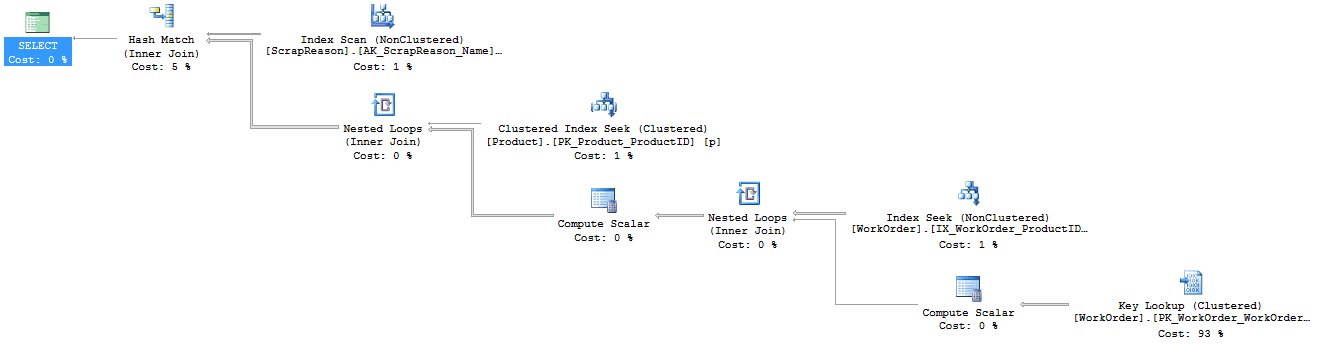
Figure 1 (Click on image for full size)

Each symbol in the execution plan is an operator, and each operator has additional information within its Properties that define the work performed by that operator. In Figure 1, we can see that in order to fulfill this query, SQL Server needs to perform two separate Compute Scalar operations. These are calculations being performed on the data as it gets retrieved. Figure 2 shows the Defined Values list from the Properties of the first Compute Scalar operator, directly after the Key Lookup.

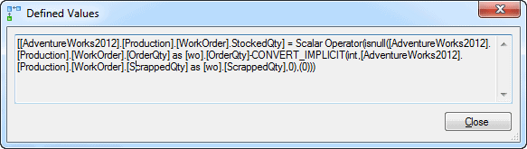
Figure 2

We can now see that, in order to arrive at a value for StockedQty, SQL Server needs to perform a calculation. This isn’t necessarily a problem, but it does demonstrate the ‘hidden work’ that SQL Server needs to perform to execute a query, which is not evident when just looking at the query alone.

Speaking of extra work, that Key Lookup operation represent extra work that we can help SQL Server avoid. The key lookup operation shows that SQL Server has to retrieve data the clustered index on the WorkOrder table because the non-clustered index on that table is not a covering index, meaning it doesn’t satisfy all the needs of the query. We could possibly improve performance by modifying that non-clustered index.

What is your ORM Tool Doing?

Object Relational Mapping (ORM) tools are pretty amazing. That’s right, I’m a DBA and I support the use of ORM tools. Oh, I know the horror they can inflict on an unsuspecting database, but that’s not the tool’s fault. If you choose to attempt to hammer in a bolt, prepare for messy results; it’s not the fault of the hammer.

In my experience, 90-98% of all queries generated by ORM tools are fine. They’re well-structured and perform perfectly well. The other 2-10% can cause issues. Severe issues. These are queries that not only “look funny” to a DBA’s eyes, but also don’t optimize well and perform extremely poorly.

When using an ORM tool, you should use some type of tool to capture performance metrics. The best of these tools will also show you if the performance problems are within the application code or the database. I work for Red Gate so perhaps I’m biased, but I do recommend ANTS Performance Profiler for exactly this type of work.

Using the performance metrics, you can identify those slow spots where the queries are not performing to specification, and then drill down into those queries and identify what’s happening in their execution plans. These plans will tell you how SQL Server’s query optimizer is resolving the ORM-generated SQL. Depending on what you find, you may need to modify your ORM-generated code in order to tune the SQL statement, or you may need a stored procedure. Yes, the point of using an ORM is to avoid manual coding of SQL, but that doesn’t mean we can never, ever, manually code. There are places where it makes sense. The good news is, at the most, that’s probably only about 10% of the time.

A common bit of generated code can look something like that shown in Listing 2.

Listing 2

The execution time of this query is somewhat poor. However, just by looking at the query text, it’s not evident that anything is very wrong. After all, the generated code put together appropriate JOINs and has a WHERE clause to filter data. Take a look at the execution plan though, as shown in Figure 3.

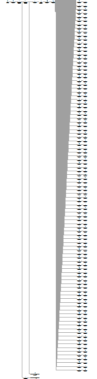
Figure 3

It’s obviously impossible to read the plan at this scale, but zooming in to a portion of the plan, as shown in Figure 4, we can see the for every parameter value within the IN clause, SQL Server performs a Constant Scan and Compute Scalar operation, to create a placeholder row and then fill in each value.

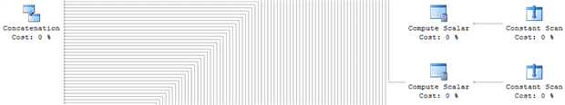
Figure 4

These values are loaded into a common stream through the Concatenation operator and then the data is sorted before it’s used in a series of joins to filter the output for return to the user.

There are a number of ways to modify the query to avoid using an IN clause. One method is to create a stored procedure that accepts a table variable (@IDList), passing the data into a table and then using that in a JOIN, as illustrated in Listing 3.

Listing 3

This change cuts execution time by three times and results in this execution plan shown in Figure 5.

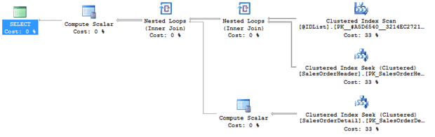
Figure 5

Examining the execution plan makes a real difference in understanding why, in this case, the generated code might be causing issues.

Query Tuning

The single largest use for execution plans is query tuning. It’s the most common tool for understanding what you want to tune. It’s invaluable for identifying and fixing poorly performing code. I can’t run through every potential cause of poor query performance here, or even close, but we can look briefly at a few of the common culprits and the warning signs you’ll find in the execution plan.

Poorly Designed Queries

Like with any language, there are common code smells within T-SQL. I’ll list out a few of them as well as what you might see in the execution plan. For more detailed examples of some of these query design problems, see my article Seven Sins against T-SQL Performance.

Search Conditions with Functions

Placing a function on a column in the WHERE, ON or HAVING clause (e.g. WHERE SomeFunction(Column) = @Value ) can lead to very poor performance because it renders the predicate non-SARGable, which means that SQL Server cannot use it in an index seek operation. Instead, it will be forced to read the entire table or index. In the execution plan, look out for a Scan operator against a table or index where you expected a Seek operation, i.e. a single or small set of lookups within an index.

Nesting Views or Nesting Functions

Having a view that calls to other views or has JOIN operations to other views can lead to very poor performance. The query optimizer goes through a process called simplification, where it attempts to eliminate tables that are not needed to fulfil the query, helping to make it faster. For simple queries involving views or functions, the optimizer will simply access the underlying base tables, and perform table elimination in the usual fashion. However, use of nested views and functions will lead quickly to a very complex query within SQL Server, even if the query looks simple in the T-SQL code. The problem is that beyond a certain point, SQL Server can’t perform the usual simplification process, and you’ll end up with large complex plans with lots of operators referencing the tables more than once, and so causing unnecessary work.

Incorrect Data Type Use

Queries can use parameters and variables in comparisons, within ON, HAVING and WHERE clauses. Unfortunately, SQL Server can only compare values of the type. For example, if you wish to compare the values in a string column (in T-SQL a VARCHAR) to the values in a DATE or DATETIME column, then you must first explicitly convert one type to match the other. If you don’t, SQL Server will perform the implicit conversion for you. When the query is executed, the query processor converts all the values of lower precedence data type, in this case the VARCHAR, to the higher precedence data type before applying the filter or join condition.

Of course, to do this it must apply the conversion function to the column, in the ON, HAVING or WHERE clause and we are back in the situation of having a non-SARGable predicate, leading to scans where you should see seeks. You may also see a warning indicating an implicit conversion is occurring.

Row-by-row Processing

SQL Server, and more specifically T-SQL, is a set-based processing system. This means it works well when the code is approached as a set.

Most developers think about processing in row-by-row terms, using loop operations. While this is perfectly correct within their normal programming environment, within T-SQL this row-by-row approach is expressed via cursors and sometimes as WHILE loops that often lead to extremely poor performance. In such cases, rather than a single execution plan, you’ll see one plan for each pass through of the loop, and SQL Server essentially generates the same plan over and over, to process each row.

Common Warning Signs in the Execution Plan

When working with execution plans, there are a few common signs of trouble. Of course, there are lots of caveats and details to be considered, but generally speaking, the following warning signs often indicate trouble spots in a query:

• Warnings – these are red crosses or yellow exclamation marks superimposed on an operator. There are sometimes false positives, but most of the time, these indicate an issue to investigate.
• Costly Operations – the operation costs are estimated values, not actual measures, but they are the one number provided to us so we’re going to use them. The most costly operation is frequently an indication of where to start troubleshooting
• Fat Pipes – within an execution plan, the arrows connecting one operator to the next are called pipes, and represent data flow. Fat pipes indicate lots of data being processed. Of course, this is inevitable if the query simply has to process a large amount of data, but it can often be an indication of a problem. Look out for transitions from very fat pipes to very thin ones, indicating late filtering and that possibly a different index is needed. Transitions from very thin pipes to fat ones indicates multiplication of data, i.e. some operation within the T-SQL is causing more and more data to be generated.
• Extra Operators – over time you’ll start to recognize operators and understand quickly both what each one is doing and why. Any time that you see an operator and you don’t understand what it is, or, you don’t understand why it’s there, then that’s an indicator of a potential problem.
• Scans – I say this all the time, scans are not necessarily a bad thing. They’re just an indication of the scan of an index or table. If your query is SELECT * FROM TableName, with no WHERE clause then a scan is the best way to retrieve that data. In other circumstances, a scan can be an indication of a problem such as implicit data conversions, or functions on a column in the WHERE clause.

Let’s take a look at a few of the warning signs that can appear, and what we can do in response. Listing 4 shows a query pattern that is fairly common, in my experience.

Listing 4

When this query is executed, you’ll see the execution plan in Figure 6.

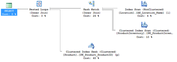
Figure 6

Several aspects of this plan give me cause for concern:

1. The Index Scan on the Location.Name column – there’s an index on that column so I’m expecting a seek
2. The fat pipe coming out of the Clustered Index Scan on the ProductInventory table – in my example, it’s processing over 1000 rows at this stage, and eventually only returning 9 rows.
3. The Hash Match join – for the number of rows returned I’m expecting a Nested Loops join.
4. The Clustered Index Seek on the Product table looks very expensive relative to the other operators – this might not be a problem but I may want to check it out

On examining the code, it’s immediately clear that the cause of the scan on Location.Name is use of a function on that column, LTRIM(RTRIM(l.Name)), in the WHERE clause. This is a common situation when developers don’t trust the consistency of the data in the column; sometimes it’s entered with trailing and leading spaces, sometimes without. The correct solution is to clean the data in the column so that it’s consistent, and use a constraint to ensure it remains so. We can then remove that function and rerun the query. On my machine, execution time went down from 156ms to 68ms, a 50% reduction. The execution plan changed as well, so that we now have an Index Seek on the Location table, as expected.

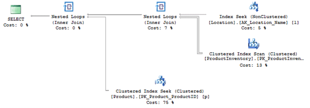
Figure 7

Also, now that the Location rows are accesses with a seek instead of a scan, SQL Server has a better idea how many rows to expect and so switches to a more appropriate join type. This is why it’s pretty common to see Hash Matches where there are bad or missing indexes.

I’m still concerned about that fat pipe connected to the Clustered Index Scan on ProductInventory, so I’m going to create a new index, as shown in Listing 5.

Listing 5

Now the fat pipe is gone, and execution time dropped even further, from 68ms to 36ms, another 50% reduction and we get a final execution plan that looks like Figure 8.

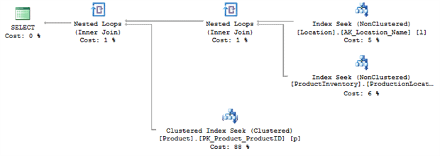
Figure 8

The final factor that may still be a concern is the high-cost Clustered Index Seek. However, once we understand the nature of the Nested Loops join, it becomes apparent that this is not actually a problem in this case. During a Nested Loops operation, for each row returned by the inner data set, in this case the 9 rows returned from the Location table, it compares it to the outer data set, looking for matches. In this case, for each row returned from Location, SQL Server performs a seek on the Product table. That explains why the cost is higher. It’s not something we need to fix because in this case, given the small number of rows involved, it’s an efficient use of resources.

Poor Indexing

If a query is running too slow, a very common solution is to add an index. But, the real question is, where do you add the index? Is it going to be to columns in the WHERE clause? What about columns in the JOIN clauses? Can you add one index for both, or will you need more than one index? If you need more than one index, how can you tell how they’re being used? The answer to all these questions is, of course, contained within the execution plan.

Being able to drill down to the execution plan after identifying a bottleneck will allow you to determine where an index is most likely to help. If you identify that a scan is taking place to return only a small number of rows then you can add an index. Having done so, you need to reexamine the execution plan to verify that the optimizer is using the new index, and using it in the way you hoped.

Referring back to the previous example, I decided to put an index on the ProductInventory table, as shown in Listing 5. Never add indexes without due consideration; always remember that for every data modification on the table, SQL Server also has to maintain all indexes on that table, which can add overhead. In this case, I chose to add one because this query will be called frequently by the application and so it needs to run as fast as possible. Therefore, any additional overhead caused by creating and maintaining an index is justified by the performance enhancement to a frequently-executed query.

The execution plan gives us quite a bit of guidance with regard to what index will be most useful and efficient. At the top of some execution plans, you may even see an explicit Missing Index suggestion, indicating that the optimizer recognized that if it had a certain index, it might be able to come up with a better plan. Note these, but do not assume they’re accurate. Test them before applying them.

In this case, there was no explicit suggestion, but we saw a Clustered Index Scan on the ProductInventory table, and by right-clicking on that operator and selecting Properties, we can reveal a lot of interesting information. Here, we’re especially interested in the Output List, i.e. the columns return by this operator, as shown in Figure 9.

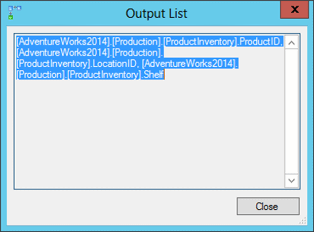
Figure 9

It outputs three columns. First is the key to the clustered index itself, ProductID. Next is the LocationID column and then finally the Shelf column.

I was using LocationID for the JOIN criteria because it’s the FOREIGN KEY constraint between the Location and the ProductInventory tables. Unfortunately, there is no index on LocationID and it needs one, which explains why I chose that column as the index key.

I also need the Shelf column from that table. If I didn’t use the INCLUDE part of the index then it would force an extra operation, a Key Lookup, to retrieve that column from the clustered index. By storing it at the leaf level with the INCLUDE clause, I avoid that extra work.

There is no need to reference the clustered key column, ProductID, in the index because it is automatically included in any non-clustered index created on that table.

This all goes together to create what is commonly referred to as a covering index, in other words, an index that completely satisfies the needs of the query without having to refer to other indexes or the table.

Misunderstanding Code Reuse in the Database

Developers are used to having code reuse built in to the object oriented programming languages they use. In SQL, they see objects such as views and user defined table valued functions and innocently assume that they are a simple means by which it promote the same sort of code reuse within the database. If they need to write a fairly complex join, write it once, store it in a view, and then whenever the application needs that data, it can just reference the view, right? From the user’s point of view this is true, but form SQL Server’s perspective, it’s a little more complicated.

A view is just a query that the optimizer resolves just like any other query. However, if you decide to JOIN a view to a view, or nest views inside of each other, it causes problems for SQL Server. Firstly, as the number of referenced objects increases, due to deep nesting, the optimizer, which only has so much time to try to optimize the query, will give up on simplification and just build a query for the objects defined. For each object, the optimizer must estimate the number of rows returned and, based on that, the most efficient operation to use to return those rows. However, once we go beyond three levels deep on obfuscation, the optimizer stops assigning costs and just assumes one row returned. All of this can result in very poor choices of plan and a lot of avoidable work.

This problem is even worse for multi-statement table valued user defined functions. These objects use the same internal structure as table variables, which means they don’t have any statistics at all. In SQL Server 2014, the optimizer will assume one hundred rows in these tables, regardless of the actual number of rows they contain. In previous versions, it assumed only a single row. This can result in execution plans that are extremely complex and, what’s more, grossly incorrect for the data being accessed.

To illustrate how nesting views can hurt the server, consider the simple query in Listing 6.

Listing 6

This would result in an execution plan as shown in Figure 10.

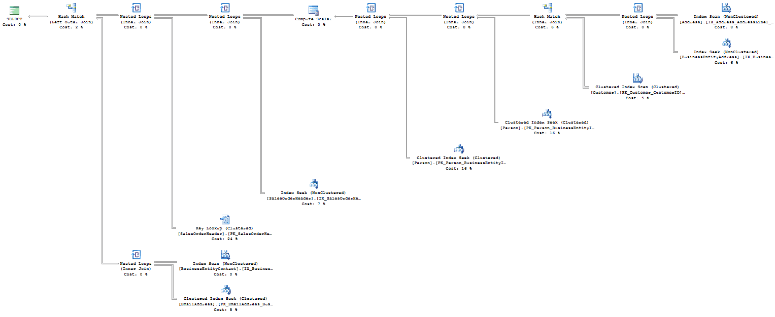
Figure 10 (Click on image for full size)

The reason this plan is so much more complicated than you might expect, for such a disarmingly simple-looking query, is because the three objects referenced are actually views with query definitions of their own, all visible through the execution plan (the view definitions are provided in the code download file accompanying this article; see the shaded box at the start of the article, to the right of the title).

Listing 7 returns similar data, and more, by accessing directly the underlying tables.

Listing 7

While a much more complex query, it actually requires a third the number of reads and executes in half the time because, instead of hitting all the tables across the entire set of views, we’ve simplified the process, manually, as you can see from the execution plan in Figure 11:

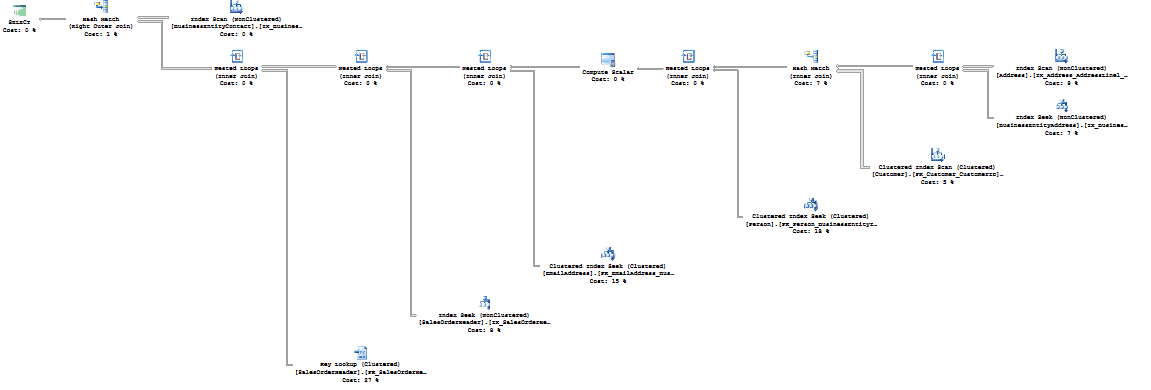
Figure 11 (Click on image for full size)

Where there were 9 tables being accessed, now there are only 8. The overall shape of the plan is simpler, and it’s a more efficient route to return the data.

In addition to the performance boost, Listing 7 also successfully returns email addresses while Listing 6 does not. This is because Listing 6 is dependent on the email addresses being listed as contacts in the BusinessEntityContact table, but no contacts within the data meet all the other criteria. By changing the JOIN criteria to reflect the fact that it’s just the BusinessEntityContact table that is preventing data from returning properly, we get a more accurate data set as well as better performance.

Database Problems outside Developer Control

Sometimes, you’re pretty sure you have your T-SQL code right, but performance is still poor. This is often caused because the optimizer has inaccurate or incomplete information about the data, and so makes poor choices of execution plan. Let’s consider a couple of different examples.

Lack of Database Constraints

One example I like to cite of SQL Server having incomplete knowledge of the data regards use of database constraints, or rather their lack of use in many databases. Consider the query shown in Listing 8.

Listing 8

With no constraints in place, the execution plan for this query will look as shown in Figure 12:

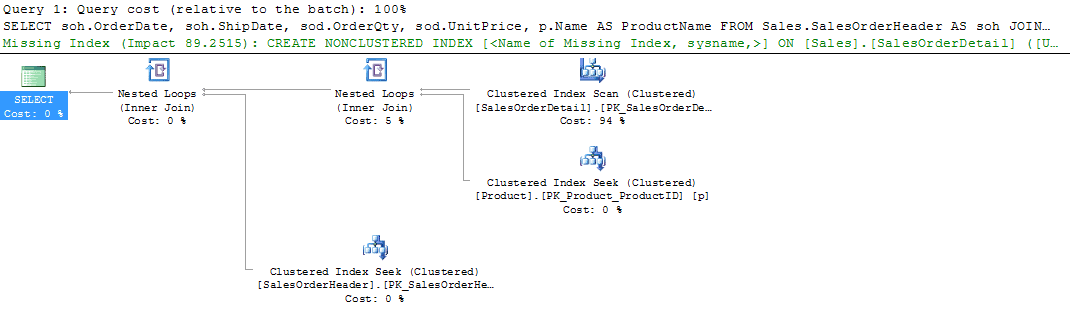
Figure 12 (Click on image for full size)

This query returns zero rows, since there are no products with a price less than $0, and yet SQL Server still performs an index scan, two index seeks and a couple of nested loop joins. The reason is that it has no way to know they query will return zero rows.

However, what if we have a constraint in place on the SalesOrderDetail table that requires that the UnitPrice for any row be greater than zero (this constraint already exists in the AdventureWorks database).

Listing 9

If we rerun Listing 8 with this constraint in place, then the execution plan, shown in Figure 13, is interesting.

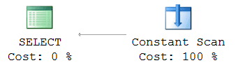
Figure 13

Again, you should not see any data returned and now, thanks to the constraint, SQL Server knows for a fact that the query cannot possibly return any rows. Therefore, rather than creating an execution plan that accesses tables that don’t need to be accessed, the optimizer correctly just creates an execution plan that creates a result set by using the Constant Scan operator, but that result set is empty and always will be.

This illustrates another interesting aspect of how the optimizer makes choices based on the object definitions within your database and the T-SQL code you supply to it. Those choices are only visible through the execution plan.

Missing or out-of-date Database Statistics

Another common cause of bad plans, due to database “configuration problems”, is insufficient or inaccurate information about the volume and distribution of the data in the database. If you learn how to spot the warning signs in the plan, you can bring up the matter with your DBA!

A common cause of the optimizer having ‘bad’ information about the data is stale statistics. The execution plans in SQL Server show us how the data is being retrieved, including how many rows of data the query optimizer thinks it might find and, if you have an actual execution plan, how many rows the SQL Server engine found. If you find that the estimated number of rows and the actual number of rows within a plan are wildly different, it suggests you have issues with statistics, or, once again, the T-SQL code.

Let’s take a look at an example of the problems causes by stale statistics. Consider the query in Listing 10.

Listing 10

This query results in the execution plan shown in Figure 14.

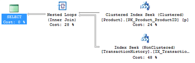
Figure 14

This plan makes a lot of sense. We’re not dealing with very many rows, SQL Server performs seeks against the indexes, and it returns the data in about 30ms. To show what happens with out of date statistics, run the script in Listing 11.

Listing 11

This script turns off the automatic update of statistics on the server. Then, within a transaction that I rollback so that I don’t affect the underlying data permanently, I modify the data in the table on order to make all the rows match the search condition in our query, instead of just a few. Figure 15 shows the first execution of the original query, after updating the data.

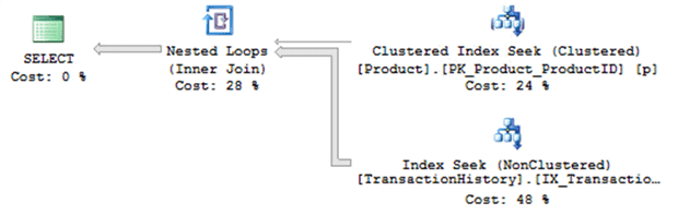
Figure 15

This plan is identical to the previous plan, except for one thing: the pipes are much fatter, especially the one between the TransactionHistory index seek and the Nested Loops operator. The statistics did not get updated after we ran the UPDATE and so SQL Server was unaware the data had changed, and so reused the same plan as before.

Click on the pipe with the Properties window open, or hover your mouse over the pipe and look at a Tooltip, and you can see information about the data flowing through the pipe. This shows the disparity between the estimated number of rows and the actual number of rows as shown in Figure 16.

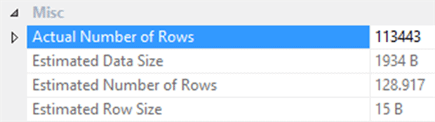
Figure 16

The Actual Number of Rows is 113,443 while the Estimated Number of Rows is 128.917 (proving this is an estimate since you can never have a fraction of a row).

Next in the script in Listing 11 you’ll see that I manually update the statistics for the table that I modified so that, now, the statistics will no longer be out of date. The next execution of the query results in a different execution plan, shown in Figure 17.

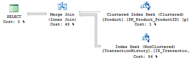
Figure 17

The principal difference is the use of the Merge Join instead of the Nested Loops. Now that SQL Server knows that many more rows will be returned, is selects a join type more dutiable to dealing with that volume. A Merge Join takes the sorted output from two sources and very efficiently combines them together.

The real difference though is the execution times. The execution of the original query, with a plan based on out of date statistics, takes about 606ms on my system. The execution using the new query plan, based on current statistics takes 500ms, almost 20% improvement.

As you can see, the execution plan reflects the state of the database almost directly and will provide you with adequate information to understand that state, as long as you take the time to read through the plan.

Maybe it’s not the Database?

Heretical thought for most developers, I know, but sometimes the problem is with the application, not the database, or the database code. If you’re only returning a few rows from the database as defined by the execution plan without scans or any other indication of a problem, there’s a good chance, the slow performance might be elsewhere. This is when it really helps to have application and code measurement metrics in addition to any metrics for measuring the database performance. A tool such as Ants Performance Profiler, as mentioned earlier, will profile both your .NET code and SQL code, and will allow you to view execution plans for any seemingly-problematic queries.

It’s All About Knowledge

I’ve met developers who feel that to spend time ‘mucking around’ within the database and looking at execution plans is an unnecessary distraction from the task of coding the essential business logic. Personally, however, I’m firmly behind the idea that developers should absolutely be looking at some of the internals of SQL Server, using execution plans.

Understanding only comes through knowledge. Sure, you don’t need to learn all the guts of the SQL Server engine to write good application code, but when your application code runs into issues with the database, you need an understanding of just what is happening in the database, and the execution plans supplied by SQL Server can provide that understanding.

Your increased understanding of how the database works, will be reflected in the other code you write and even your ability to support the business through applications. We’re moving rapidly into a new world. There’s a lot more bleed-over between what used to be the carefully delineated roles of database administrator and developer. The movement towards application lifecycle management (ALM), DevOps and database lifecycle management (DLM) within ALM, all strongly suggest that developers need to have a better understanding of what their code actually does within the database.

Therefore, you have every reason to learn execution plans and hopefully, this article has got you started. If you’re keen to learn more, you might want to check out my SQL Server Execution Plans book (available as a free eBook download).