
The series so far:
- Creating Calculated Columns Using DAX
- Creating Measures Using DAX
- Using the DAX Calculate and Values Functions
- Using the FILTER Function in DAX
- Cracking DAX – the EARLIER and RANKX Functions
- Using Calendars and Dates in Power BI
- Creating Time-Intelligence Functions in DAX
If you should ever start reading a book on DAX, you will quickly reach a chapter on the CALCULATE function. The book will tell you that the CALCULATE function is at the heart of everything that you do in DAX and is the key to understanding the language. A delegate on one of my courses adopted the policy of starting every formula with =CALCULATE, and it’s not such a bad approach! This article explains how to use the CALCULATE function and also how to use the (almost) equally important VALUES function.
The Example Database for this Article
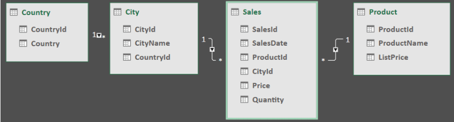
This article uses the same simple database as its two predecessors. This database shows sales of three toys for different cities around the world:
You can import this data into your own Power BI data model by first downloading this Excel workbook, or by running this SQL script in SQL Server Management Studio.
As for the previous articles in this series, everything I describe below will work just as well in Power BI, PowerPivot or Analysis Services (Tabular Model), each of which Wise Owl train.
The CALCULATE Function
To understand the CALCULATE function, you must understand filter context, so that’s where I’ll begin for this article.
Filter Context Explained Using an Excel Pivot Table
Suppose you have the following pivot table in Excel, showing the number of sales for each country, city, and product in the database. The figure selected shows that there were three sales of Timmy Tortoise products in London (UK):
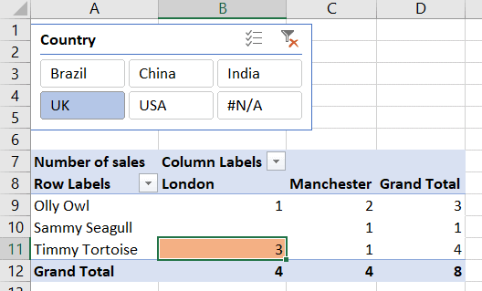
The filter context for the shaded cell containing the number 3 is therefore as follows:
Country dimension: UK
City dimension: London
Product dimension: Timmy Tortoise
If you were to double-click on this cell in Excel, you would see the underlying rows:
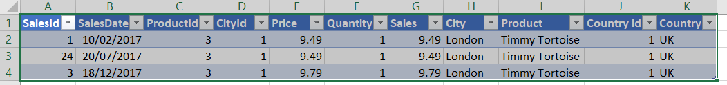
These are the three sales which took place for this product in this country and city.
Now suppose that you change your pivot table to show the number of sales as a percentage of the total for each column. This would give:
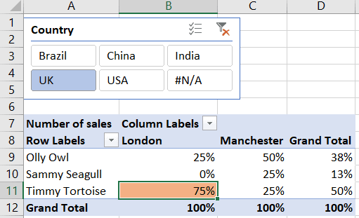
The figure for Timmy Tortoise for London is 75%, which is:
|
1 2 |
Total sales for London for Timmy Tortoise / Total sales for London for all products |
This gives 75% because this is the result you get when you divide 3 (the number of sales in London for Timmy Tortoise) by 4 (the number of sales in London for all products).
Note that I’ll often refer in this article to the numerator and denominator. In any fraction A / B, the numerator is A and the denominator is B (but you knew that from school maths, didn’t you?).
Removing One Constraint Using CALCULATE and ALL
Now suppose that you want to recreate this pivot table using a matrix and slicer in Power BI:
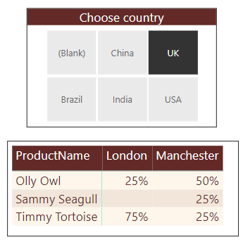
The figures are exactly the same, and for Timmy Tortoise for London you’ll see 75% because this is the ratio between the number of sales for this product and city (3) against the number of sales for all products and this city (4).
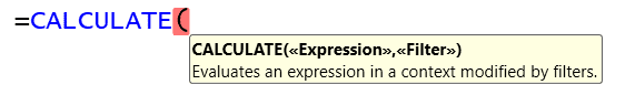
To solve this problem, you’ll use the CALCULATE function which is the answer to most questions in DAX. The syntax of the function is as follows:
The measure you should create (and show) is this:
|
1 2 3 4 5 6 7 8 9 10 11 |
% of all products = DIVIDE( // the numerator: number of sales for the current filter context COUNT(Sales[SalesId]), // the denominator: number of sales for the current filter // context, but for ALL products CALCULATE( COUNT(Sales[SalesId]), ALL('Product'[ProductName]) ) ) |
I’ve put my measure in a separate table – if you’re not sure how to create this table or how to create measures, see the previous article in this series. What the measure does is to calculate the numerator (the number of sales for the current product and city) and divide this by the denominator (the number of sales for the current city only, with any product constraint removed). Here’s what this calculates:
|
1 2 3 |
Total sales for the current filter context / Total sales for the current filter context, but removing any product constraint |
If you display row and column totals for this measure, you get this:
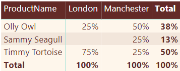
The figures in the bottom row make sense: total sales for London for all products divided by total sales for London for all products will always give 100%!
Removing Multiple Constraints Using ALL
Suppose that you now want to display the number of sales as a percentage of the total for all cities and for all products, to get this:
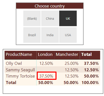
In this case, the numerator is the total number of sales in the UK in London for Timmy Tortoise, and the denominator is the total number of sales in the UK; the other two constraints have been removed from the denominator. Here is a DAX measure to calculate these figures:
|
1 2 3 4 5 6 7 8 9 10 11 12 |
% of all products and cities = DIVIDE( // divide the number of sales ... COUNT(Sales[SalesId]), // ... by the number of sales for all products and // cities CALCULATE( COUNT(Sales[SalesId]), ALL('Product'[ProductName]), ALL(City[CityName]) ) ) |
You can use the ALL function as many times as you like – each time it will remove one dimension from the filter context.
Using ALLEXCEPT to Remove All but One Constraint
An alternative solution to the above problem would be to calculate this ratio:
|
1 2 3 |
Total sales for the current filter context / Total sales for the current filter context, but removing every constraint apart from the country one |
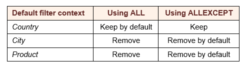
Here’s a quick comparison of the two approaches:
Here’s a measure which would show each product/city’s contribution to the grand total for each country:
|
1 2 3 4 5 6 7 8 9 10 11 12 13 14 |
% relaxing everything but country = DIVIDE( // divide the number of sales ... COUNT(Sales[SalesId]), // ... by the number of sales, keeping only the // country constraint CALCULATE( COUNT(Sales[SalesId]), ALLEXCEPT( Sales, Country[CountryName] ) ) ) |
It’s up to you whether you think it’s more elegant to remove constraints from the filter context individually using ALL, or to remove all constraints apart from one using ALLEXCEPT.
Replacing Filter Context Using CALCULATE
The previous examples have all involved removing the filter context in whole or in part. What if you wanted to change it to show the ratio for each matrix cell between the number of sales for that cell and the number of sales for the same filter context, but for the product Timmy Tortoise? That is, you want to calculate:
|
1 2 3 |
Total sales for the current filter context / Total sales for the current filter context, but ignoring any product constraint and using the Timmy Tortoise product instead |
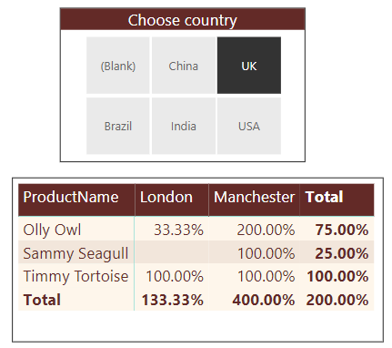
For this example, it’s inevitable that the figures for Timmy Tortoise should be 100%, because for each cell in this row you’re dividing a figure by itself. The matrix above shows that sales of Olly Owl were only a third of those for Timmy Tortoise in London but were twice those for Timmy Tortoise in Manchester.
A formula that you could use might be:
|
1 2 3 4 5 6 7 8 9 10 11 12 |
% of Timmy = DIVIDE( // divide the number of sales for the filter context by ... COUNT(Sales[SalesId]), // ... the number of sales for the filter context, but // removing any product constraint and replacing this // with a constraint that the product should equal Timmy Tortoise CALCULATE( COUNT(Sales[SalesId]), 'Product'[ProductName] = "Timmy tortoise" ) ) |
What this does is to calculate the number of sales for a particular country, city and product, and divide this by the number of sales for the same country and city, but for Timmy Tortoise. The extra filter you add in the CALCULATE formula doesn’t build on the filter context for the product, but instead replaces it.
Using the ALLSELECTED Function as Opposed to ALL
Sometimes you’ll want to reference just the selected items in a dimension, in a slicer, for example, rather than include all of the items in your formula. Here’s an example of a matrix where you might want to do this:
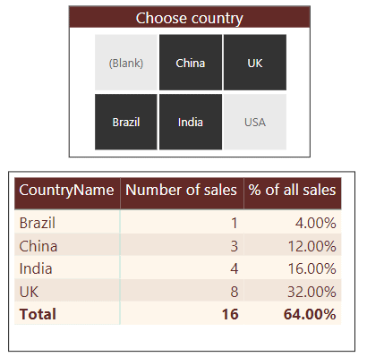
The measure shown initially is as follows:
|
1 2 3 4 5 6 7 8 9 10 |
% of all sales = DIVIDE( // divide number of sales for filter context ... COUNT(Sales[SalesId]), // ... number of sales for all countries CALCULATE( COUNT(Sales[SalesId]), ALL(Country[CountryName]) ) ) |
The figures don’t add up to 100% because for each country the statistic shown equals:
|
1 2 |
the number of sales for that country / the number of sales for all countries |
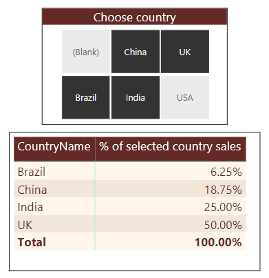
In this example the USA is included in the denominator but not in the numerator. To get the statistic to work, you need to reference only the selected countries in the denominator:
|
1 2 3 4 5 6 7 8 9 10 11 |
% of selected country sales = DIVIDE( // take the number of sales for each country COUNT(Sales[SalesId]), // divide this by the number of sales for all // currently selected countries CALCULATE( COUNT(Sales[SalesId]), ALLSELECTED(Country[CountryName]) ) ) |
This gives the required 100% total, regardless of the combination of countries you select in the slicer:
Context Transition Using the CALCULATE Function
Before moving on from the CALCULATE function, it has one more string to its bow. Consider the following two formulae:
|
1 2 |
Total sales A = SUMX(Sales,[Price]*[Quantity]) Total sales B = CALCULATE(SUMX(Sales,[Price]*[Quantity])) |
If you’ve been following up to now, you’ll realise that these two formulae must give the same result under all circumstances:
The first formula gives the total sales value for the current filter context;
The second formula gives the total sales value for the current filter context, with no extra modifications to it.
However … what happens if there isn’t a filter context to begin with? In this case the second formula will create a filter context, and hence return a different answer than the first. How can you not have a filter context? By creating a calculated column in a table:
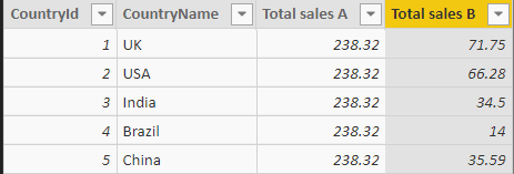
The first formula gives the same result for each row. Because calculated columns don’t have a filter context by default, the formula sums sales over all of the rows in the sales table, giving the same answer (238.32) for each.
Remember that the second formula is as follows:
|
1 |
Total sales B = CALCULATE(SUMX(Sales,[Price]*[Quantity])) |
The CALCULATE function doesn’t just allow you to change the filter context, it can create it, too. For each country, this creates a filter context, limiting the rows in the sales table to those for the country in question, and hence giving a different answer for each row of the above table. The process of changing row context into filter context in this way is called context transition.
The VALUES Function
Learning the CALCULATE function is key to understanding how to create measures in DAX, but the VALUES function runs it a close second. The rest of this article shows what this function does, and how to use it to create a range of effects in your Power BI reports.
What the VALUES function returns
The VALUES function returns the table of data for the current filter context. To explain what this sentence means, here’s an example. Suppose you create this table in a Power BI report:
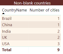
Note for this example that I’ve used a filter (not shown here) on the report to avoid showing any blank countries). The Number of cities column shows the number of cities for each country, using the following measure:
|
1 |
Number of cities = COUNTROWS(VALUES(City[CityName])) |
If you could look at the filter context, this is what you would see:
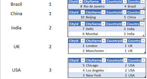
The VALUES function allows you to return a table containing one or more of the columns in the current filter context’s underlying table. For example, you could create this measure:
|
1 |
Cities = VALUES(City[CityName]) |
If you display this measure in your Power BI report, you’ll get this error message:
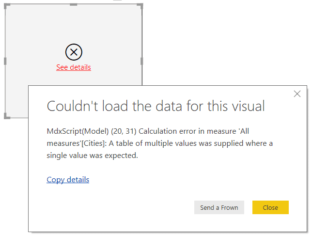
The problem is that you’re trying to display a column of values in a single cell. This would work for Brazil and China, each of which only has one city, but wouldn’t work for the other three countries.
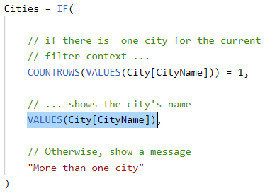
What you could do, however, is to test whether there is only one city for a country, and in this event show its name; otherwise, you could show a message saying that there are multiple cities. Here’s a measure to do this:
|
1 2 3 4 5 6 7 8 9 |
Cities = IF( // if there is one city for the current // filter context ... COUNTROWS(VALUES(City[CityName])) = 1, // ... shows the city's name VALUES(City[CityName]), // Otherwise, show a message "More than one city" ) |
Displaying this measure in our report would give:
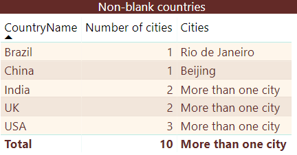
For the total row there are lots of cities in the current filter context, so naturally you get the More than one city message.
The above example shows two important features of the VALUES function. The first is that it returns a table of data. In the measure above, the COUNTROWS function expects to receive a table:
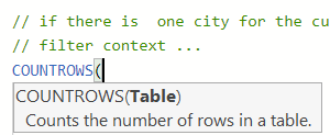
Fortunately, that’s what’s supplied:
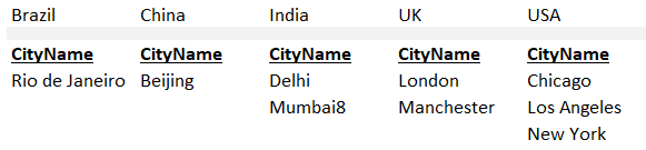
The VALUES function in this case returns a single-column table which looks like this for each of the 5 countries:
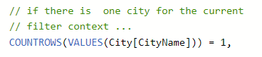
The second important point to understand about the VALUES function is that you can’t put a table into a cell without performing some sort of aggregation on it first, since a table can potentially contain multiple values. What this means is that the selected part of the measure below shouldn’t work:
This is because the VALUES function returns a column of data, and even though you know that there is only one row in this column, and hence only one value, you would normally still need to apply some aggregation function (e.g., MAX, MIN, SUM) to the data.
Happily, there is one exception to this rule. If a call to the VALUES function returns a table with one column and one row, you can automatically treat this as a single scalar value without any additional work. This is why this measure works!
The HASONEVALUE Function and Other Alternatives
Checking whether the filter context only contains one value for a particular column is a common thing to do. It’s so common, in fact, that DAX has a dedicated function called HASONEVALUE to do this.
You could rewrite the measure like this:
|
1 2 3 4 5 6 7 8 9 |
Cities = IF( // if there is one city for the current // filter context ... HASONEVALUE(City[CityName]), // ... shows the city's name VALUES(City[CityName]), // Otherwise, show a message "More than one city" ) |
Another solution would be to count how many distinct city names there are in the current filter context:
|
1 2 3 4 5 6 7 8 9 |
Cities = IF( // if there is one city for the current // filter context ... DISTINCTCOUNT(City[CityName]) = 1, // ... shows the city's name VALUES(City[CityName]), // Otherwise, show a message "More than one city" ) |
These three methods, using VALUES, HASONEVALUE or DISTINCTCOUNT, are interchangeable, and I don’t think there’s any clear reason to favour one over another.
Using CONCATENATEX to List Out Multiple Values
For this example, you might want to list out the names of the cities for each country. You can do this using the CONCATENATEX function, which has this syntax:
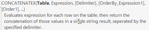
The arguments to this function are thus:
- The table containing the values you want to concatenate
- The column in this table containing the values to concatenate. You have to specify this even if the table only has one column, even though in this case it is blindingly obvious that this is the one you should choose!
- The text you want to use as glue to join the column values together
- Which column you want to order by. Again you need to specify this, even if you know you’re working with a single-column table.
- The order-by direction, ascending or descending
For this example, you could modify the measure to read like this:
|
1 2 3 4 5 6 7 8 9 10 11 12 13 14 15 |
Cities = IF( // if there is one city for the current // filter context ... DISTINCTCOUNT(City[CityName]) = 1, // ... shows the city's name VALUES(City[CityName]), // Otherwise, list all city names CONCATENATEX( VALUES(City[CityName]), City[CityName], ",", City[CityName], ASC ) ) |
This more or less works, since it gives this table:
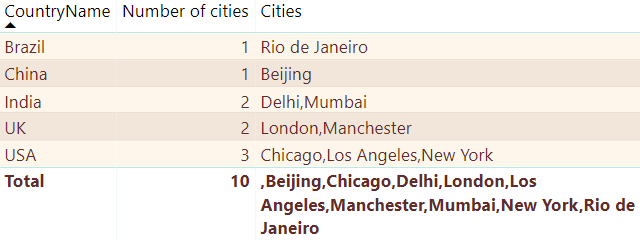
The only remaining problem is that the total row now looks odd. Technically it is correct, because, for this row, the filter context contains all of the cities for all countries. A better solution would be to check whether there is more than one country in the filter context:
|
1 2 3 4 5 6 7 8 9 10 11 12 13 14 15 16 17 18 19 20 21 22 |
Cities = IF( // if there's only one country in the filter context ... HASONEVALUE(Country[CountryName]), // ... show the city name or names ... IF( // if there is one city for the current // filter context ... DISTINCTCOUNT(City[CityName]) = 1, // ... shows the city's name VALUES(City[CityName]), // Otherwise, list all city names CONCATENATEX( VALUES(City[CityName]), City[CityName], ",", City[CityName], ASC ) ), // ... or otherwise show nothing BLANK() ) |
This is what you should now see when using this measure in the table:
All of this illustrates an important point about DAX measures. You can create a measure which gives sensible results for one particular visual, but can you be sure that it will give sensible results in another? Or in a totals row? Or a totals column, or grand total? You’ll often be faced with a trade-off in DAX between checking that a measure works under all possible circumstances and keeping things simple.
Modifying the Filter Context Using VALUES
Suppose that you now want to display the total sales for each country apart from the UK. The obvious way to do this is to sum total sales, but using the CALCULATE function to amend the filter context to omit the UK:
|
1 2 3 4 5 6 7 8 9 |
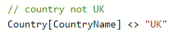
Value of sales = CALCULATE( // calculate total sales value SUMX( Sales, [Price] * [Quantity] ), // country not UK Country[CountryName] <> "UK" ) |
This suffers from one major problem – it doesn’t work! Displaying this measure in a table would show the same value for every country:
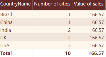
To understand why this measure is showing 166.57 for every country, remember what I said earlier in this article: when you apply a filter, it replaces the current filter context for a dimension. For this example you’re adding this filter to the CALCULATE function:
What this does is to lose any existing filter by the country dimension and replace it with one where the country is UK. Here’s what’s going on for each country:
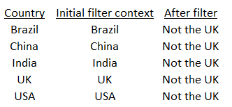
The total sales value for all of the countries apart from the UK is 166.57, so that’s what gets displayed in every row. What you want to do is to keep the existing filter context constraints for the country dimension, but then add to them. One way to do this is to use the VALUES function, making the new measure read like this:
|
1 2 3 4 5 6 7 8 9 10 11 |
Value of sales = CALCULATE( // calculate total sales value SUMX( Sales, [Price] * [Quantity] ), // keep the country filter as it is VALUES(Country[CountryName]), // and add that the country should not be the UK Country[CountryName] <> "UK" ) |
This would give the following results:
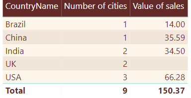
If you’re wondering why there is a discrepancy between the 166.57 shown in the first table and the 150.37 shown in the second, it’s explained by the fact that I had filtered the table to remove any sales taking place with no assigned country. If you remove this filter you get:
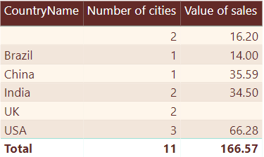
Add these 16.20 of sales in as above and you would get the required figure.
Using Disconnected Slicers to Make Reports Dynamic
This is a clever idea, which allows you to make reports dynamic. The idea is to create a slicer which allows you to choose which measure you want to show. In the example below, someone has chosen to show the average price of sales:
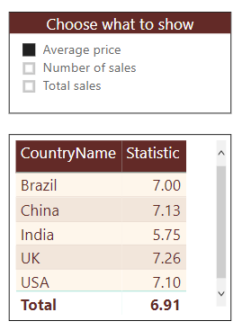
To make this work, first create a table to hold the statistics that you might want to report:
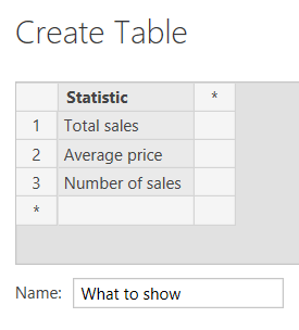
However, don’t link this table to any other. That’s why this technique is often called a “disconnected slicer”. Now create a slicer based upon this table:
The idea is that when you select a statistic in the slicer, the bottom table will show its value. All that you now need to do is to create and show a measure which will yield:
- The average price of sales if someone selects the first measure;
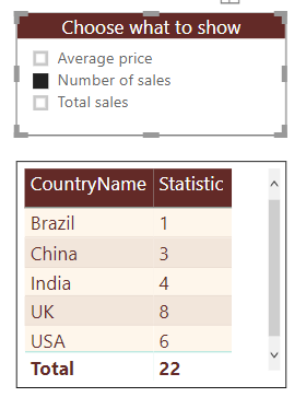
- The number of sales records if someone selects the second measure;
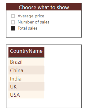
- The total value of sales if someone selects the third measure; or
- A blank if someone selects more than one statistic at a time or doesn’t select one at all.
Here’s what this measure might look like!
|
1 2 3 4 5 6 7 8 9 10 11 12 13 14 15 |
Statistic = // first find out what user wants to see (assume one thing chosen) VAR Choice = SELECTEDVALUE('What to show'[Statistic]) // return different measure according to choice RETURN IF( HASONEVALUE('What to show'[Statistic]), SWITCH ( Choice, "Average price", AVERAGE(Sales[Price]), "Number of sales", COUNTROWS(Sales), "Total sales",SUMX(Sales,[Price]*[Quantity]) ), BLANK() ) |
One final question: is it possible to display different statistics using different number formatting? I can’t think of any way to do this except to use the FORMAT function:
|
1 2 3 4 5 6 7 8 9 10 11 12 13 14 15 16 |
Statistic = // first find out what user wants to see (assume one thing chosen) VAR Choice = SELECTEDVALUE('What to show'[Statistic]) // return different measure according to choice RETURN IF( HASONEVALUE('What to show'[Statistic]), SWITCH ( Choice, "Average price", FORMAT(AVERAGE(Sales[Price]),"0.00"), "Number of sales", FORMAT(COUNTROWS(Sales),"#,##0"), "Total sales",FORMAT(SUMX(Sales,[Price]* [Quantity]),"#,##0.00") ), BLANK() ) |
The problem with this is that the FORMAT function turns numbers into text, although because it does so only after the calculation is complete for each filter context, this shouldn’t cause too much of a problem. Here’s what you’d see for the number of sales for the above measure, for example:
And just in case you’re wondering, I can’t think of any way to change the column title dynamically!
Dynamic Titles
There’s one more thing to demonstrate with the creative use of the VALUES function: how to show the choices made in a slicer. For the report page below, you’d like a card visual (shown selected) to display a measure listing the countries chosen:
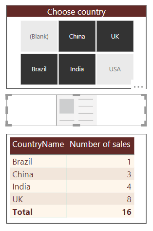
Here are some examples of what the card should display:
- For the choices shown above, it should read “Brazil, China, India, UK”
- If a user doesn’t select a country, it should read “All countries”
- If a user picks a single country, it should give the country’s name
If you’ve been following the article so far, there’s nothing new with this – it just combines lots of the ideas you’ve already seen. Here’s a measure which would fit the bill:
|
1 2 3 4 5 6 7 8 9 10 11 12 13 14 15 16 17 18 19 20 21 22 23 |
Title = IF( // if there are countries selected ... ISFILTERED(Country[CountryName]), // test to see if one, or more than one IF( HASONEVALUE(Country[CountryName]), // there's one country selected; show it (but must use // the VALUES function to convert the single column, // single row table into a scalar VALUES(Country[CountryName]), // otherwise, join the country names together CONCATENATEX( Country, Country[CountryName], ",", Country[CountryName], ASC ) ), // if we get here, then user didn't select // any countries "All countries" ) |
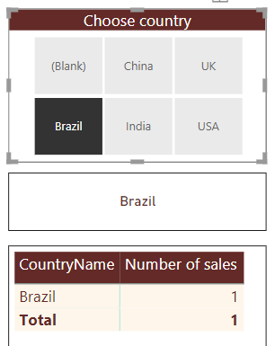
Here’s what this would show if you have one country selected assuming that you attach the measure to your card:
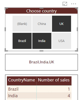
If you have multiple countries selected, you’ll see this:
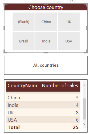
And finally, if you have no countries selected, you’ll see this:
If you want to be even fancier you could use a quick measure to display only the first 3 countries in any list which I covered in the previous article in this series.
Conclusion
This article has shown how you can use two of the most important DAX functions: CALCULATE and VALUES. The article began by showing how you can use the CALCULATE function to amend the default filter context, mainly in order to create ratios. I then showed how you can use functions like VALUES, HASONEVALUE and ISFILTERED to produce a variety of clever effects in DAX. The next article in this series will look at the FILTER and EARLIER functions. You should make sure that you understand clearly how you can use the CALCULATE function to change filter context before progressing, since the DAX formulae won’t get any easier!