In my last article, “Getting Started with the SSAS Tabular Model,” I introduced you to the SQL Server Analysis Services (SSAS) tabular database and how to access its components in SQL Server Management Studio (SSMS). This article continues that discussion by demonstrating how to use the Data Analysis Expressions (DAX) language to retrieve data from your tabular database.
DAX has a rather unique history in that it’s a formula language with its roots in PowerPivot, an in-memory data exploration tool that brought the tabular model to Excel. In fact, DAX is often considered an extension to the formula language used in Excel.
When Microsoft added support for the tabular model in SSAS 2012, they included support for both DAX and Multidimensional Expressions (MDX), the language traditionally used to access SSAS multidimensional data. You can use either DAX or MDX to query data in an SSAS tabular database. However, you cannot use MDX if the database is configured to run in DirectQuery mode. In addition, some client applications, such as Power View, can issue DAX queries only. As a result, if you plan to support tabular databases, you should have at least a basic understanding of how to use DAX to access data in those databases.
Because DAX has its roots in PowerPivot, much of what has been written about the language has focused on how to create expressions that define measures and calculated columns. But there might be times when you want to use DAX to access data directly from a tabular database, either by issuing queries in SSMS or by creating them in other client applications. This article explains how to get started writing DAX queries within SSMS and provides numerous examples that demonstrate each concept. For these examples, we use the AdventureWorks Tabular Model SQL 2012 database, available as a SQL Server Data Tools tabular project from the AdventureWorks CodePlex site.
Retrieving Table Data
To query data in an SSAS tabular database from within SSMS, you must first connect to the SSAS instance that contains the database and then open an MDX query window. You have to use an MDX query window because SSMS currently does not support a DAX-specific query window. However, you can write DAX queries directly in the MDX window without taking any other steps.
When using DAX to retrieve tabular data, your entire statement is founded on the evaluateevaluateevaluateInternetSales table:
|
1 2 3 4 |
evaluate ( 'Internet Sales' ) |
Figure 1 shows part of the results returned by this statement. There are in fact, many more columns and rows than what are shown here. But as you can see, using an evaluate clause to retrieve all of a table’s contents is a simple and straightforward process.
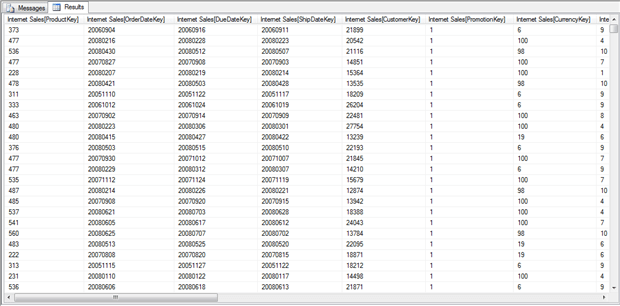
Figure 1: Retrieving all data from the Internet Sales table
In addition to the evaluate clause, you can also specify an order by clause that sorts your result set. For example, the following statement includes an order by clause the sorts the results based on the ProductKey column of the InternetSales table:
|
1 2 3 4 5 6 |
evaluate ( 'Internet Sales' ) order by 'Internet Sales'[ProductKey] |
Notice that you first specify the order by keywords, followed by the column name on which you want to order the data. If can include more than one column, but you must separate them with a comma. When specifying the column name, you must precede it with the table name, enclosed in single quotes, and then the column name, enclosed in brackets. This method of referencing a column is typical of the approach you generally use when referencing columns in your DAX statements. With the addition of the order by clause, the results are now sorted by the ProductKey column, as shown in Figure 2.
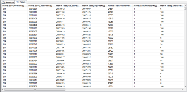
Figure 2: Ordering a result set based on the ProductKey values
As handy as it is to be able to pull all the data from a table, more often than not you won’t want to. For instance, at times you’ll likely want to retrieve only specific columns. Unfortunately, DAX makes retrieving only some table columns a less than straightforward process, so you must use a workaround to get the information you need. One of the easiest solutions is to use the summarize function. This function groups data based on specified columns in order to aggregate data in other columns, similar to how a GROUP BY clause works in a T-SQL SELECT statement.
However, you can also use the summarize function to return all rows in a table without grouping any of the data. To do so, you must first include a column or columns that uniquely identify each row in the table. For example, the following evaluate clause uses the summarize function to retrieve the Sales Order Number and Sales Order Line Number columns:
|
1 2 3 4 5 6 7 8 9 10 11 12 |
evaluate ( summarize ( 'Internet Sales', 'Internet Sales'[Sales Order Number], 'Internet Sales'[Sales Order Line Number] ) ) order by 'Internet Sales'[Sales Order Number], 'Internet Sales'[Sales Order Line Number] |
When you use the summarize function, you specify the function name and then the arguments passed into the function. The first argument is your base table. All subsequent arguments are the columns you want to include in the result set. As you can see in the above example, the arguments are enclosed in parentheses and separated with commas.
The summarize function groups the data by the values in the specified columns. However, together the Sales Order Number and Sales Order Line Number columns uniquely identify each row in the table, so all rows are returned and no values are grouped or summarized. Notice, too, that the order by clause now includes the two columns specified in the summarize function, separated by a comma. Figure 3 shows some of the rows returned by the DAX statement:
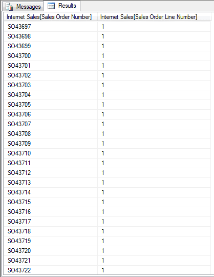
Figure 3: Retrieving distinct values from a table
If you were to scroll down these results, you would find a number of repeating Sales Order Number values, but each set of the repeated values would include unique Sales Order Line Number values, which is what makes each row unique. In other words, no two rows would share the same Sales Order Number value and the same Sales Order Line Number value.
Of course, you’re likely to want to include additional columns as well, once you’ve identified the columns that uniquely identify each row, in which case, you need only add those columns to the mix. In the following example, the ProductKey and OrderDate columns have been added to the summarize function:
|
1 2 3 4 5 6 7 8 9 10 11 12 13 14 |
evaluate ( summarize ( 'Internet Sales', 'Internet Sales'[Sales Order Number], 'Internet Sales'[Sales Order Line Number], 'Internet Sales'[ProductKey], 'Internet Sales'[Order Date] ) ) order by 'Internet Sales'[Sales Order Number], 'Internet Sales'[Sales Order Line Number] |
As you can see in Figure 4, the results now include the additional columns, sorted by the Sales Order Number and Sales Order Line Number columns.
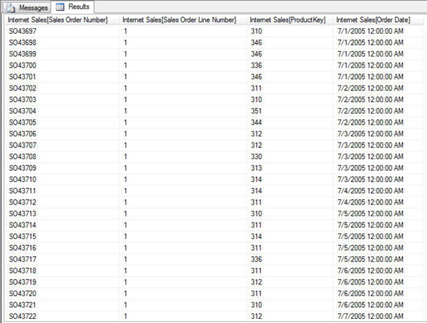
Figure 4: Retrieving specific columns from a table
The examples so far have demonstrated how to return all rows in a table. However, the nature of SSAS and the tabular model suggest that, in many cases, you’ll want to work with summarized data. After all, conducting meaningful analysis often depends on the ability to aggregate large datasets. And the summarize function can help perform much of that aggregation. So let’s take a closer look at that function.
Summarizing Data
As mentioned earlier, the columns you specify in the summarize function form the basis of how the data is grouped. In the previous two examples, we chose columns that uniquely identified each row, so no real grouping was performed, at least not in the sense that one would expect from a function used to group and summarize data. However, suppose we were to now remove the Sales Order Number and Sales Order Line Number columns, as shown in the following example:
|
1 2 3 4 5 6 7 8 9 10 11 12 13 |
evaluate ( summarize ( 'Internet Sales', 'Internet Sales'[ProductKey], 'Internet Sales'[Order Date], "Total Sales Amount", sum('Internet Sales'[Sales Amount]) ) ) order by 'Internet Sales'[ProductKey], 'Internet Sales'[Order Date] |
As you can see, this time round we’re grouping our data on the ProductKey and Order Date columns only, and we’re also doing something else, adding a third column that aggregates the data.
The new column is considered a calculated column (or extension column). When adding a calculated column in this way, we include two parts. The first is the name of the new column (Total Sales Amount), enclosed in double quotes. The second part is an expression that defines the column’s values. In this case, we’re using the sum aggregate function to add together the Sales Amount values. To do so, we need only specify the function name, followed by the column, enclosed in parentheses. Now our results include three columns, with the values grouped together by the ProductKey and Order Date columns and the amount of sales for each grouping added to the Total Sales Amount column, as shown in Figure 5.
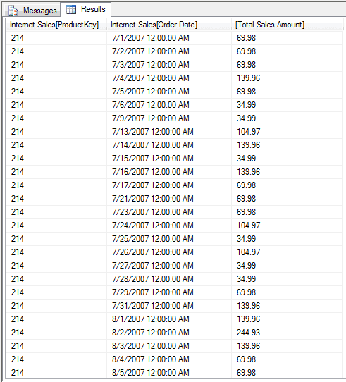
Figure 5: Summarizing data in a table
As you can see, DAX lets us easily get the data we need from our table. However, you might find that you want to include columns from other tables in your result set, as you would when joining tables in a T-SQL SELECT statement. Fortunately, DAX and the tabular model makes it simple to retrieve these columns. For example, suppose we want to retrieve the product names instead of the product numbers and the order year instead of a specific date and time. We can easily achieve this by modifying our summarize function as follows:
|
1 2 3 4 5 6 7 8 9 10 11 12 13 |
evaluate ( summarize ( 'Internet Sales', 'Product'[Product Name], 'Date'[Calendar Year], "Total Sales Amount", sum('Internet Sales'[Sales Amount]) ) ) order by 'Product'[Product Name], 'Date'[Calendar Year] |
As you can see, in place of the ProductKey column, we now have the Product Name column from the Product table, and instead of the Order Date column we have the Calendar Year column from the Date table.
NOTE: Pulling data from the Calendar Year column in this way masks the fact that multiple relationships exist between the Internet Sales table and the Date table. The first of these relationships is defined on the OrderDateKey column in the Internet Sales table. As a result, the Calendar Year value returned by our statement is based on the date represented by that key. An explanation of the logic behind all this is beyond the scope of this article, but know that what we’ve done in our example serves its main purpose: to demonstrate how easily we can retrieve data from other tables.
In addition to switching out columns, we’ve also updated our order by clause to reflect the new columns. Now are results our substantially different, as shown in Figure 6.
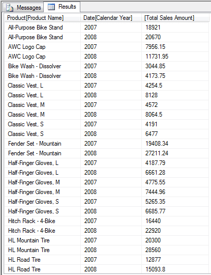
Figure 6: Retrieving data from other tables
As you can see, we’ve grouped our data first by product name and then by the calendar year, with sales totals provided for each group. If you were to scroll down the list, you would find that our results include other years as well. Not surprisingly, these results are much quicker to comprehend because they include easily identifiable information: the product names and sales years.
In addition, we can easily add more columns. The following example is similar to the last but now includes the Product Subcategory Name column from the Product Subcategory table and the Product Category Name column from the Product Category table:
|
1 2 3 4 5 6 7 8 9 10 11 12 13 14 15 16 |
evaluate ( summarize ( 'Internet Sales', 'Product'[Product Name], 'Product Subcategory'[Product Subcategory Name], 'Product Category'[Product Category Name], 'Date'[Calendar Year], "Total Sales Amount", sum('Internet Sales'[Sales Amount]), "Total Cost", sum('Internet Sales'[Total Product Cost]) ) ) order by 'Product'[Product Name], 'Date'[Calendar Year] |
You might have noticed that we also added a second calculated column named Total Cost. For this column, we add the values in the Total Product Cost column for each of our groupings. Figure 7 shows part of the results returned by our updated DAX statement.
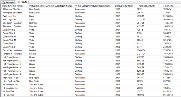
Figure 7: Retrieving additional columns from a table
Another option that the evaluate clause supports is the ability to roll up our results based on our grouping. To do so, we use the ROLLUP function on the column whose totals we want to roll up. For example, in the following DAX statement, the evaluate clause includes the ROLLUP function applied against the Calendar Year column:
|
1 2 3 4 5 6 7 8 9 10 11 12 13 14 15 16 |
evaluate ( summarize ( 'Internet Sales', 'Product'[Product Name], 'Product Subcategory'[Product Subcategory Name], 'Product Category'[Product Category Name], ROLLUP('Date'[Calendar Year]), "Total Sales Amount", sum('Internet Sales'[Sales Amount]), "Total Cost", sum('Internet Sales'[Total Product Cost]) ) ) order by 'Product'[Product Name], 'Date'[Calendar Year] |
To use the ROLLUP function, you need only to precede the column name with the function name and enclose the column name in parentheses. As you can see in Figure 8, our results now include an additional row for each product. The new row provides totals for that product for all years.
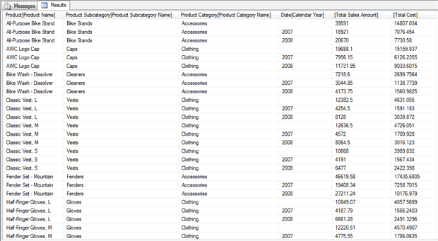
Figure 8: Using the ROLLUP operator to summarize data
Not surprisingly, there’s far more you can do when using DAX to summarize data, but what we’ve covered here should help you get started. And you’ve seen how specific we can be in terms of which columns we return. So now let’s look at how we can filter data even further.
Filtering Data
One of the easiest ways to filter data in a DAX statement is to use the filter function. The function takes two arguments: a table expression and a filter. The table expression can be the name of a table or an expression that returns a table. The filter is a Boolean expression that is evaluated for each row returned by the table expression. Any row for which the expression evaluates to true is included in the result set.
Let’s look at an example to better understand how the filter function works. In the following evaluate clause, the filter function filters data in the Internet Sales table:
|
1 2 3 4 5 6 7 8 9 |
evaluate ( filter ( 'Internet Sales', 'Internet Sales'[Sales Amount] > 1000 ) ) order by 'Internet Sales'[ProductKey] |
The first argument in the filter function is the name of the table, and the second argument is the Boolean expression, which specifies that the value in the Sales Amount column must be greater than 1000 for the row to be returned. As a result, all other rows are filtered out. However, because we’ve specified the Internet Sales table as our table expression, the result set still includes all columns from that table.
Instead of specifying a table name as our first argument in the filter function, we can specify a more specific table expression. In the following example, we use the summarize function as our table expression:
|
1 2 3 4 5 6 7 8 9 10 11 12 13 14 15 16 17 18 19 20 |
evaluate ( filter ( summarize ( 'Internet Sales', 'Product'[Product Name], 'Product Subcategory'[Product Subcategory Name], 'Product Category'[Product Category Name], 'Date'[Calendar Year], "Total Sales Amount", sum('Internet Sales'[Sales Amount]), "Total Cost", sum('Internet Sales'[Total Product Cost]) ), 'Date'[Calendar Year] > 2006 ) ) order by 'Product'[Product Name], 'Date'[Calendar Year] |
The summarize function should look familiar to you. It pulls product and sales information from several tables. We then filter the data based on the Calendar Year column so that our results include only those years after 2006.
Adding Columns
At times, you might want to add columns to a table without grouping or summarizing that data. One way to do this is to use the addcolumns function, as shown in the following example:
|
1 2 3 4 5 6 7 8 9 10 11 12 13 14 |
evaluate ( filter ( addcolumns ( 'Product', "Net Profit", 'Product'[List Price] - 'Product'[Standard Cost] ), 'Product'[List Price] > 0 ) ) order by 'Product'[ProductKey] |
In our example, we once again we start with a filter function, but this time, as our first argument, we use the addcolumns function to return a table. The addcolumns function takes as its first argument a table or table expression. In this case, we’re using the Product table. After we specify our table, we add a definition for a calculated column, just like we did with the summarize function. In this case, however, the column is named Net Profit, and the column’s values are based on an expression that subtracts the Standard Cost value from the List Price column. We then filter our results so that only rows with a List Price value greater than 0 are included in the result set. Figure 9 shows part of the results returned by the DAX statement. Notice the Net Profit column added after all the table’s other columns.
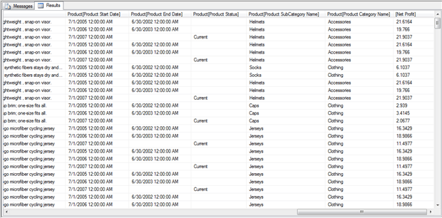
Figure 9: Adding columns to a table
Of course, you’ll often want to be more specific with your table expression, rather than simply returning the entire table. For example, you can use the summarize function as your table expression. In fact, the addcolumns function can be particularly helpful when used in conjunction with the summarize function.
Let’s take a step back. As you’ll recall from earlier examples, we used the summarize function to add the Total Sales Amount and Total Cost computed columns to our result set. However, in some cases, you’ll see better performance if you use the addcolumns function to create those columns, rather than creating the computed columns within the summarize function, as shown in the following example:
|
1 2 3 4 5 6 7 8 9 10 11 12 13 14 15 16 17 18 19 20 21 22 23 |
evaluate ( filter ( addcolumns ( summarize ( 'Internet Sales', 'Product'[Product Name], 'Product Subcategory'[Product Subcategory Name], 'Product Category'[Product Category Name], 'Date'[Calendar Year] ), "Total Sales Amount", calculate(sum('Internet Sales'[Sales Amount])), "Total Cost", calculate(sum('Internet Sales'[Total Product Cost])) ), 'Date'[Calendar Year] > 2006 ) ) order by 'Product'[Product Name], 'Date'[Calendar Year] |
In this case, the summarize function specifies only the columns on which to group the data. The function returns a table as the first argument to the addcolumns function. We can then add our computed columns as arguments to the addcolumns function. The only thing to remember, however, if we add columns in this way and those columns aggregate data, we must also use the calculate function to call our aggregated column. (This has to do with the context in which DAX evaluates data.) Figure 10 shows part of the results returned by the DAX statement.
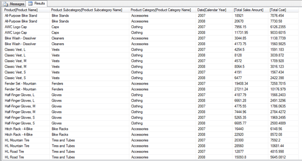
Figure 10: Adding columns when summarizing data
Using the addcolumns function to add computed columns works in most, but not all, situations. For example, you cannot use this approach when you want to use the ROLLUP function. (Be sure to check the DAX documentation for specifics on when to use addcolumns.) However, when you can use the addcolumns function in conjunction with the summarize function, you should see better performance.
Moving Ahead with DAX
Now that you’ve gotten a taste of how to use DAX to retrieve tabular data, you should be ready to start putting DAX to work. Keep in mind, however, that what we’ve covered here only scratches the surface of what you can do with DAX. It is a surprisingly rich language that includes a number of methods for retrieving and summarizing data. In future articles in this series, we’ll look at how to access a tabular data from other client applications, often using DAX in the process. What you’ve learned in this article should provide you with the foundation you need to facilitate that data access. Keep in mind, however, that the better you understand DAX, the better you’ll be able to make use of your tabular data.