The previous article in this project, Set-based Thinking, discussed why a set-based approach is much faster and less resource-hungry than a RBAR-approach, for accessing data rows. In this article, I am going to demonstrate why storing data in an efficient manner, for both saving and fetching rows, is very important in terms of data integrity and, to a certain point, query performance.

We’ll create a completely de-normalized design and then work through the refactoring process necessary to transform the design, step-by-step, through each of the Normal Forms. At each stage, we’ll assess the impact of our changes on query design and performance, and in terms of the reduction in exposure to the risk of data modification anomalies.

To work through the example in this article, you will need the set of scripts available at the bottom of the article, as well as a means to generate one million rows of test data. I used SQL Data Generator (and provide my SDG project file with the download), but other tools are available.

Table Design in OLAP versus OLTP

An OLAP (Online Analytical Processing) system is typically subject to few writes and many reads. For example, a data warehouse is an OLAP system where data storage is centralized and refreshed one or more times per day. The number of reads is high, because the data warehouse’s fact-tables hold all historical data. Built on top of the data warehouse are reports, in Reporting Services, and cubes, in Analysis Services, for examining historical trends, predicting future ones, and so on.

When designing tables for such a system, we want the tables to be as wide as possible to save CPU when reading the data; in other words, we want to denormalize the data as far as possible, to save computation time for JOINs.

By contrast, OLTP (Online Transaction Processing) systems are typically subject to many writes and fewer reads. For these systems to be as effective as possible, the guidelines for table design, to ensure speed and accuracy, are very different but equally important. Here, we would like our database to be normalized, as far as is practical.

Problems with De-normalized Designs

A typical de-normalized database design will generally contain only a few, large tables with many columns. These tables are likely to contain data that is not well structured. For example:

• A column may contain compound values, requiring SQL Server to perform often-complex calculations to return the required data
• A column may contain redundant data (a strong indicator that a database is under- normalized is the need to use the DISTINCT keyword in SQL queries, in order to return the correct data set).

There are several well-documented problems with such designs, relating to data integrity. Consider, for example, the de-normalized Articles table shown in Figure 1, which stores various details regarding each product, along with the target customer group.

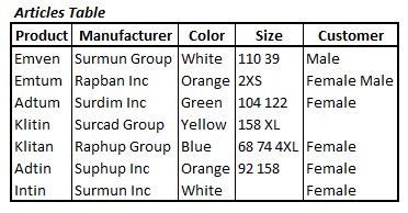
Figure 1: The de-normalized Articles table (0NF)

I have seen tables like this many times, in the work of novice database designers. The benefit is that it is human-readable and so it is easy to find the information we want, just by looking at the table. However, it is a design that flouts many of Chis Date’s five guidelines to help design normalized tables:

1. There is no top-to-bottom ordering to the rows
2. There is no left-to-right ordering to the columns
3. There are no duplicate rows
4. Every row-and-column intersection contains exactly one value from the applicable domain (and nothing else)
5. All columns are regular (no hidden row IDs, object IDs, or timestamps)

As a result, it is a design that suffers from redundant data storage, and is vulnerable to accidental deletes and updates, as well as data modification anomalies.

For example, if Surmun Inc. stopped making the product Intin in the color white, someone might simply delete that seventh row from the database. In doing so, they would remove Intin as a product as well as Surmun Inc as a manufacturer (assuming this was the only row that referenced either), and so lose any record of this product in our system.

The Size and Customer columns store multiple sizes and multiple target customer groups, respectively. This design flouts Date’s Rule 4, which states that all data values should be atomic. For certain reports, or when working with a data warehouse, it may make sense from a performance perspective to pre-aggregate data to concatenated strings. However, for any OLTP database, storing multiple values in same column is counter-productive.

Finally, by flouting Date’s Rule 4, we are also likely to break Rule 3. For example, we may have two rows that that identical values in all columns, except Size, where one row lists sizes “104 122” and another lists sizes “122 104”. We, as humans, know that this is a duplicate row, but the database cannot tell. This means that whenever we make a modification to the data in this table (e.g. to list Adtum as Maroon rather than Green), we’d need to be sure to make the change to all the duplicate rows.

By normalizing the database design, splitting the entities into separate tables, we gain more control over the data and safeguard against these, and other, potential data integrity issues. As a considerable fringe benefit of this process, our queries will be easier to write and understand and, up to a point, will perform a lot better, especially in cases where the row count runs into millions. Consider, for example, the Size column in the de-normalized Articles table. It will require use of costly and time-consuming string manipulation algorithms when inserting and deleting sizes. In addition, to answer a simple question such as, “Can I have an Adtum in size 122?” our query would need to perform a scan of the Articles table looking for references to “122” in the Size column, if present at all. No index here will help us speed up this query.

Database Normalization: the Road to Third Normal Form

Dr Edgar Frank Codd wrote the first rules of normalization when working for IBM in the 1970’s. Later, together with Chris Date, he helped formalized the 12 rules for how a Database Management System (DBMS) should be designed to be relational (RDBMS).

Excluding a few variants, there are six Normal Forms, from First Normal Form (1NF) to Sixth Normal Form (6NF), which when applied successively to a database design will help remove redundancy and dependency.

In a de-normalized design, many set-based querying techniques will be inapplicable, indexes will be ineffective, and almost every query against the table will need to scan the complete table. The result, in my experience, is that the developer turns to use of cursors, and other forms of RBAR (row-by-agonizing-row) coding, rather than the set-based approach.

By applying normalization techniques, set-based querying becomes easy and we utilize the full power of the RDBMS (including indexes). As such, normalization will, up to a point, improve the performance of most queries, as well as offer protection from data modification anomalies, make it easier to expand the design, and so on.

When most people refer to a database as “normalized”, they mean that it adheres to Third Normal Form (3NF). In some ways, 3NF is the unofficial Normalization threshold and, for most applications, designing the database for adherence to higher Normal Forms would be over-normalization in that it will not add significant value (which is not to say that it is never necessary).

A database that adheres to 3NF will be one in which (among other things):

• Each table describes a separate entity – making it easier to extend an application’s functionality without having to redesign all the tables
• Data redundancy is eliminated – reducing the possibility of data anomalies during modification
• We can exploit the power of set-based querying – for example: a query performs a simple aggregation over a certain time-period; if there were no events over that period, we still want to return a row (with a zero count). With a normalized design, this becomes possible, using an OUTER JOIN to the “dimension” table.

Note that when the design achieves 3NF, our tables will automatically also adhere to 1NF and 2NF. However, there is no guarantee that 3NF also obeys higher Normal Forms (it depends on the application requirements).

Over the coming sections, we will start with a completely de-normalized database design and then normalize it in steps, through 1NF to 5NF, and examine the effect on query design and performance, as well as on data storage and redundancy. Before we start, I’ll add the disclaimer that an online search will reveal a number of subtly different interpretations of the different Normal Forms.

Denormalized Design (0NF)

Our 0NF design consists of the single Articles table from Figure 1. In order to follow along, you will need to create a sample Articles table (see Listing 1) and then populate it with some sample data.

Listing 1: Creating the 0NF articles table

I used Red Gate’s SQL Data Generator to load the data, creating a table containing 1 million rows of data, which is small enough for performance testing. For those who have the tool, or opt to download the 14-day trial version, I’ve provided the SDG project that I used (you’ll need to open it with an XML or Text editor, such as EditPad, and change the SQL Server connection details).

We can now design some queries to answer the following common “questions”, which may be asked of our data:

• Find the number of unique products
• Find the number of unique pink colored Products, targeted for Males in Size 122
• Find the number of unique sizes

Listing 2 shows the code required to answer these questions, for our 0NF design.

Listing 2: 0NF queries

Notice that to return the number of products all three queries use the DISTINCT keyword, which I highlighted as a warning earlier in the article. Also, note the inelegant search condition in Query 2, necessitated by the fact that the size and customer might be part of a “composite” value. In Query 3, we have to use a special-purpose fnParseList function in order to separate the composite data into single values.

Just from the standpoint of query complexity, I hope you can see, already, that there are good reasons to normalize our tables. By calculating the permutations over Size and Customer columns, we realize quickly just how much information is stored in a table. Figure 2 shows the performance metrics (CPU, Duration and Reads) for each of these queries. Of course, your metrics may differ, depending on the data created in your setup.

Figure 2: 0NF query performance

In each case, the query will have needed to scan the complete table in order to return the desired results. Notice that both Query 1 and Query 2 perform the same number of reads even though the latter returns less than a tenth of the number of rows. This is explained, by the difficulty involved, for the RDMBS, in evaluating the WHERE clause, and the work required to remove all duplicates, with the DISTINCT keyword. Query 3 is painfully slow even for this relatively small number of rows, due to need to parse the Size column.

Let’s now move on and normalize our design to 1NF, rewrite our queries to return the same results, and compare performance.

First Normal Form (1NF) – Eliminate repeating groups

Eliminating repeating groups is a relatively simple step, achieved by creating a separate table for each set of related attributes (i.e. grouping the attributes into entities), and identifying each row with a unique column (or set of columns), i.e. giving each table a primary key.

So, how do we identify repeating groups? A repeating horizontal group is easy to spot. Let’s say the designer had chosen the alternate design for our Articles table, shown in Figure 3.

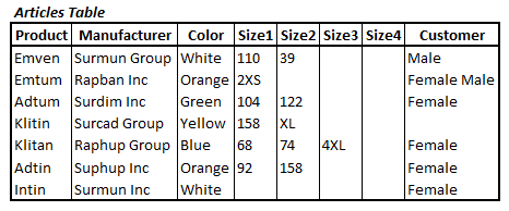
Figure 3: An alternative design for the Articles table, with a repeating horizontal group

This design has four “Size” columns, one for each size. It eliminates the problem of compound values in a single row-column intersection, but this new design makes it very hard to answer questions like “which other products from Suphup Inc come in size 92?” The query would look something like that shown in Listing 3.

Listing 3: A query dealing with repeating groups

This query would be very inefficient and get more inefficient the higher the number of Size columns.

In the 0NF Articles table in our example (Figure 1), the designer has chosen to avoid repeating horizontal groups by allowing a single Size column to store multiple sizes, flouting Date’s fourth rule. This de-normalized Articles table, in effect, still has repeating horizontal groups; the delimiter is just a space and not a pair of CRLF characters. However, while this is a problematic design, for reasons we’ve already discussed, this type of repeating group does not break the compliance rules for 1NF, so we don’t have to fix it at this stage.

However, the same issues, namely the 1-to-many relationship between Products and Sizes (a product comes in many sizes), is likely to cause repeating vertical groups. If multiple personnel maintain the inventory, then it’s likely that some might enter as a new row, data for a product with the same manufacturer and color as an existing product, but a different size, whereas others could simply add the new size to the Size column for an existing row.

Therefore, if the intended candidate key for Articles table is { Product, Manufacturer, Color}, then it is highly likely this key will contain duplicates (i.e. repeating vertical groups). We must fix this issue in order for the design to comply with 1NF. In addition, we have the problem that Product is not dependent on Size because some products may have no size (conversely, size is always bound to a product).

Therefore, our first job is to create a separate entity for products, by splitting the Articles table and creating a new Products table, as shown in Figure 4. A Product always has a Manufacturer and a Manufacturer always has a Product so we will not yet split these entities.

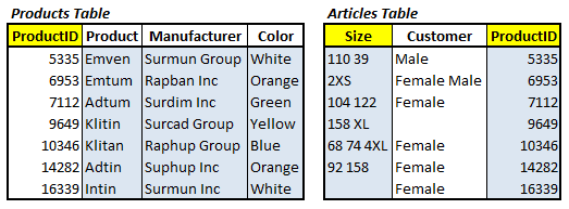
Figure 4: The 1NF Design (Yellow is Primary Key, Blue is candidate key)

Our new Products table must comply with Date’s five rules, meaning that it cannot contain composite information nor duplicate information.

The code to convert the design from 0NF to 1NF, and transfer the necessary data, is provided in in the script 0NF-1NF.sql, available as part of the code download. I won’t reproduce this code in the article, but will explain the major refactoring steps.

The first task is to create the new Products table, as shown in Listing 4. Note that we create a surrogate key on the Products table, via a new IDENTITY column, called ProductID.

Listing 4: Creating the new Products table

We also need to identify, for our new Products table, a candidate key, i.e. a column, or combination of columns, which can identify a row as unique and distinct from other rows in same table, according to the business rules. In our example, with the existing columns, the candidate key is a composite key comprising the { Product, Manufacturer and Color } columns. In the script, I create a unique clustered index based on these three columns. For some other application or business requirements, the Color may also be part of the candidate key, but in this example, it is not. In my script, I have added an index over Color column to speed up some queries.

As discussed, there is no guarantee that the combination of those three keys, in the existing Articles table, uniquely identifies a row, so when populating the Products table, in the script, we need omit duplicates. Having done this, we can create a FOREIGN KEY constraint between Products table and Articles table, based on the ProductID column, and then drop the Product, Manufacturer and Color columns from the Articles table.

In our Articles table, which currently still flouts Date’s rules, the candidate key, and primary key, is a composite of Size and ProductID. SQL Server does not accept nullable columns as part of the primary key, so we simply update any NULL values in the S ize column to an empty space, and then make the resulting Size column non-nullable.

Natural or Surrogate keys?

The choice of natural versus surrogate key is mostly a matter of preference. Some purists will tell you to use only natural keys, but there are cases where natural keys cannot guarantee uniqueness. The classic example is Social Security Number (SSN); it’s a good candidate for a natural key, but the fact is that a) not everyone has a SSN, b) SSN is not guaranteed to be unique and c) an SSN may change, for example due to a gender change or a person joining a witness protection program. Whatever you choose, make sure the primary key is smaller than the size of the candidate key in the source table. There is nothing to gain from making the the new key larger than the combined size of the candidate key. In most cases, a surrogate key is smaller than a natural key.

Benefits of 1NF over 0NF

With the design changes we have made so far, the Products table now complies with all five of Date’s rules. Some of the benefits of the 1NF design, over 0NF, are obvious:

• Our candidate key on the Products table ensures that we have no duplicates, so any changes will only need to be made in one place
• We can now remove rows from the Articles table without losing the product, manufacturer and color information
• Our foreign key protects us from accidentally deleting the row, say with ProductID 7112 from the Products table (unless the FK constraint is set to ON CASCADE DELETE).

Note, though, that the design is still not free from the risk potential update anomalies. For example, if Rapban Inc manufactures Emtum in multiple colors, then a change in product name will require someone to update all occurrences in order to avoid anomalies.

Let’s look at the impact of this new design on how we write our queries, and on the performance of those queries. Listing 5 shows the new queries.

Listing 5: 1NF queries

Notice that Query 1 is now very straightforward, and does not require use of the DISTINCT keyword. However, we still need the DISTINCT keyword for queries 2 and 3 because the Size (and Customer) values can appear in duplicate.

Figure 5 shows the performance of these queries, compared to their 0NF counterparts.

Figure 5: 1NF query performance, compared to 0NF

Note that before we worry about performance improvements, it’s very important to check that, in all three cases, the 1NF queries return exactly the same number of rows as their 0NF counterparts.

Query 1 now performs substantially faster due to eliminating the repeating vertical groups. Query 2 has to perform fewer reads but has temporarily got slower because we’ve introduced a JOIN, and not yet fixed the problems with the Size and Customer columns.

The performance of Query 3 has improved only slightly, again due to removal of eliminating the repeating vertical groups, while not yet fixing the composite nature of the Size column.

Second Normal Form (2NF) – Eliminate Redundant Data

For our design to conform to 2NF, we must move to a separate table any attribute that depends on only part of a composite key. In the Products table, we have a composite key composed of { Product, Manufacturer and Color}. However, the name of the product is depends only on the identity of that product, and the same argument applies to manufacturer and color. This leads to redundant data storage; for example, every time we add a new color for an existing product we have to re-list, redundantly, the name of the product and the manufacturer of that product. In order to resolve this issue, we must move each component of the composite key to a separate table.

Similarly, for the Articles table, every row redundantly lists all target customers and all sizes and so we should move the Size column to a separate table. Note that we don’t yet move the Customer attribute to a separate table since it doesn’t contribute at all to the key in Articles table. Figure 6 shows the resulting 2NF design.

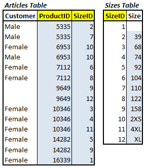
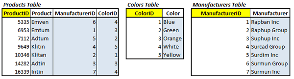
Figure 6: The 2NF Design

Again, every new table we create must obey Date’s five rules, so in order that our new Sizes table will comply, we need to deal with the composite values in the Size column. Performing this split, populating the Sizes table with unique sizes, and creating the Foreign key relationship to the Articles table requires a complex series of steps that I’ll allow you to examine in the 1NF-2NF.sql script, rather than reproduce them here.

Having done this, we recreate the Articles table with the candidate key, and the primary key, being a combination of ProductID column and the new Size ID column. As part of this step, we fix the Customer column to remove duplicates.

In our new 2NF design, we again chose to introduce a surrogate keys as the Primary Keys for each of the new Sizes, Colors, and Manufacturers tables. This is just a matter of preference. However, surrogate keys have a tendency to be smaller and more efficient in terms of space occupied in the table and indexes.

This 2NF design is a big improvement over 1NF, in terms of protection from modification anomalies, and offers other advantages over the 1NF design. Let’s consider, for example, a new business requirement to store Warranty information. In the 1NF design, where each row listed all size and customer information, this request could have represented difficulties. How would we handle it, for example, if the warranty were different depending on size? In the 2NF design, we have a lot more flexibility in terms of how to implement this change. We can now choose whether to add the new Warranty column to the Product table or the Article table, or both.

Again, having performed the refactoring, we examine the impact of this new database design on the design and performance of our three queries. Listing 6 shows the new queries.

Listing 6: 2NF queries

Figure 7 shows the performance of these queries, compared to their 0NF and 1NF counterparts.

Figure 7: 2NF query performance, compared to 1NF and 0NF

Notice that Query 1 and Query 2 didn’t gain much from higher normalization, but Query 3 did! In the 1NF design, the response time for Query 3 was about 3 minutes, whereas in 2NF, it is instantaneous. In addition, the read count went down from about 12 million to two, which is about 6 million times less reads!

It seems likely that Query 1 and Query 3 have reached their peak performance, or close, and so we can predict that further normalization will not lead to any significant further improvement in performance. However, it is obvious Query 2 might benefit from further normalization.

There is also another very good reason to continue with the normalization process and that is to further preserve data quality and prevent of accident updates or deletes.

Third Normal form (3NF) – Eliminate columns not dependent on keys

In order for our design to comply with 3NF, we must move any columns that do not contribute to the key into a separate table. For our example, it means that we should move the Customer column out of the Articles table, into its own table as shown in Figure 8.

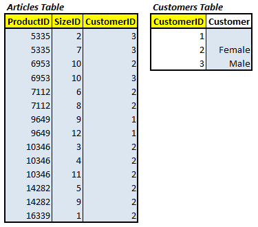
Figure 8: The 3NF Database Design

All of the changes needed to convert our 2NF design into the 3NF design are set out in the script 2NF-3NF.sql, available as part of the code download. As you will see, we have to do some significant work on the Articles table, in order to make this change, and that was to change NULL values to an empty space. This means that we would have to re-code any front end to deal with this new behavior, where “empty space” means “no value”.

Again, let’s look at the impact of this new design on query design and performance. Listing 7 shows the 3NF version of the queries.

Listing 7: 3NF queries

Figure 9 shows the performance of these queries, compared to their 2NF counterparts.

Figure 9: 3NF query performance, compared to 2NF

The performance of query 2 has improved significantly over the 2NF design (even though it performs more reads). However, Queries 1 and 3 perform comparably to 2NF.

At this point, I get most objections from my customers when I suggest normalization to them. “Why should we have to write so much more code to get the same result and comparable performance?”

My answer is that writing code is a one-time operation, whereas “data quality” is always on going. If your priority is for the coders to be “done” as quickly as possible, go with the de-normalized approach. However, bear in mind that your tables are likely, over time, to acquire duplicate data, requiring use of DISTINCT for almost all queries, even something as simple as summing up a total stock value. Your data will also be susceptible to accidental UPDATE and DELETE operations, and extending the design (for example to add a Warranty” column) will be hard.

If you want maintainable tables and high performance queries, choose the normalized approach. Your coders will take a few seconds or minutes more to write the queries, but the queries will run faster (up to a point) and your data will be stable and free from anomalies. Adding a “Warranty” column will be easy to do.

Beyond 3NF

Over the course of refactoring our database design from 0NF to 3NF, we massively improved the performance of all three of our queries. We are now at the “end of the road” in terms of performance benefits of further normalization and, for most applications, will have sufficiently normalized to preserve data quality, so it’s time to stop normalizing.

So why do the other, higher Normal Forms exist? The short answer is that they deal with certain “permutations of attributes”. In our example, this means permutations of the Product, Customer and Size attributes. Not all permutations may exist; for example, some products (such as an umbrella) may have a size, but no gender-specific target customer group. Another product, such as lipstick, may have a target customer but no size.

With the 3NF design we are forced to store the non-existing counterpart for the Customer-Size permutations, and deal with the fact that some ID (in Size s table and Customer s tables) means “no value”.

In this article, I’m not going to walk through all the details of transforming the design through 4NF and 5NF. If you’re interested, the code to refactor the current 3NF design to 4NF and then 5NF is included in the code download, as are scripts containing the equivalents of our three queries, for the 4NF and 5NF designs and a separate PDF, Database Normalization: Beyond 3NF, which offers fuller details of why these higher Normal Forms might be needed.

For the record, the performance figures for the 5NF queries are very similar to those for the 3NF design, confirming that we can gain no additional performance benefits from further normalization, in this case.

How far you want to design with Normal Forms will depend on your company business requirements for the project. If you do not need it, do not design for it. If someone later tells you the business requirements have changed, you can easily start from where you left off and continue with higher Normal Form at that point.

Summary

• Separate logical entities and related attributes.
• Up to a point, a higher level of Normalization will offer both better overall performance and data quality.
• Aim for at least 3NF to be safe from accidental deletes, inserts and updates.
• Normalize not less but not more than needed.

Coming Next… Choosing the right datatype for performance, quality and accuracy.