The series so far:
- SQL Server Machine Learning Services – Part 1: Python Basics
- SQL Server Machine Learning Services – Part 2: Python Data Frames
- SQL Server Machine Learning Services – Part 3: Plotting Data with Python
- SQL Server Machine Learning Services – Part 4: Finding Data Anomalies with Python
- SQL Server Machine Learning Services – Part 5: Generating multiple plots in Python
- SQL Server Machine Learning Services – Part 6: Merging Data Frames in Python
SQL Server Machine Learning Services (MLS), along with the Python language, offer a wide range of options for analyzing and visualizing data. I covered a number of these options in the previous articles in this series and provided examples of how to use them in your Python scripts. This article builds on those discussions by demonstrating how to merge two data frames, one created from SQL Server data and the other from multiple .csv files. The final output is a third data frame that provides the foundation for plotting the data in order to generate a visualization.
The examples in this article are based on data from the AdventureWorks2017 sample database and a small set of .csv files (download at the bottom of the article) that contain data mapping back to the SQL Server data. The goal is to create a single data frame that merges the two original data sets. The final data frame will contain six years of annual sales data for a group of sales reps. The data will then be used to generate a bar chart that visualizes each individual’s sales. I created the examples in SQL Server Management Studio (SSMS), connecting to a local instance of SQL Server 2017.
Creating a data frame based on SQL Server data
As you’ve seen in the previous articles, the key to running a Python (or R) script within the context of a SQL Server database is to call the sp_execute_external_script stored procedure, passing in the Python script as a parameter value. If you have any questions about how this works, refer back to the first article in this series. In this article, we focus primarily on the Python script.
If you plan to try out these examples for yourself, you’ll ultimately create a merged data frame and use it to generate a visualization. To get to that point, you need to take four steps:
- Create the first data frame based on SQL Server data.
- Create the second data frame based on data from a set of .csv files.
- Create the final data frame by merging the first two data frames.
- Create a bar chart based on the data in the final data frame.
The following example carries out the first step:
|
1 2 3 4 5 6 7 8 9 10 11 12 13 14 15 16 17 18 19 20 21 22 23 24 25 |
Use AdventureWorks2017; GO -- define Python script DECLARE @pscript NVARCHAR(MAX); SET @pscript = N' # assign SQL Server dataset to the df1 variable df1 = InputDataSet df1["2012"] = df1["2012"].astype(int) print(df1)'; -- define T-SQL query DECLARE @sqlscript NVARCHAR(MAX); SET @sqlscript = N' SELECT TOP(6) BusinessEntityID AS RepID, LastName + '', '' + FirstName AS FullName, CAST(SalesLastYear AS FLOAT) AS [2012] FROM Sales.vSalesPerson WHERE JobTitle = ''Sales Representative'' ORDER BY SalesLastYear DESC;'; -- run procedure, using Python script and T-SQL query EXEC sp_execute_external_script @language = N'Python', @script = @pscript, @input_data_1 = @sqlscript; GO |
The example uses the sp_execute_external_script stored procedure to retrieve the SQL Server data and create the df1 data frame. As you’ve seen in the previous articles, you start by declaring the @pscript variable and assigning the Python script as its value. Next, you declare the @sqlscript variable and assign the T-SQL statement as its value. The T-SQL statement returns sales information from the vSalesPerson view. However, the statement returns only the top six rows, based on values in the SalesLastYear column, sorted in descending order. I’ve renamed the column to 2012 to indicate the year of sales. (I picked this year just for demonstration purposes. It is not meant to reflect the dates associated with the underlying data.)
With the @pscript and @sqlscript variables defined, you can then pass them in as parameter values when calling the sp_execute_external_script stored procedure. Again, refer to the first article in this series if you have questions about how any of this works.
Returning now to the Python script, you can see that it includes only a few statements. The first one assigns the data from the InputDataSet variable to the df1 variable:
|
1 |
df1 = InputDataSet |
The InputDataSet variable contains the data returned by the T-SQL statement, which is passed into the df1 variable. The df1 variable is created as a DataFrame object. You can make changes to the data frame by calling the variable. For example, the next Python statement converts the 2012 column to the int data type:
|
1 |
df1["2012"] = df1["2012"].astype(int) |
This is the first time we’ve used the astype function in this series. You call the function by tagging it onto the column reference (using a period to separate the two) and then specifying the data type. Be aware, however, when using the astype function to convert a column from float to int, Python merely truncates the values, without rounding them up or now. In this case, it’s not a big deal, but if you need more precision, you should use the round function. You can also round the values within the T-SQL statement.
That’s all you need to do to set up the first data frame. You can verify that the data frame has been created the way you want it by calling the print function and passing in df1 as the parameter value:
|
1 |
print(df1) |
The following figure shows the data returned by the print statement, as it appears in the SSMS console on my system. Your results should look similar to this.
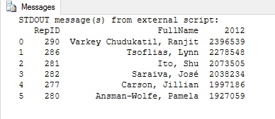
The results include the six rows returned by the T-SQL statement, with the 2012 values truncated to integers. Notice that Python automatically generates a 0-based index for the data frame, which is separate from the RepID column.
Creating a data frame based on data from .csv files
With the first data frame in place, you’re ready to create the second one. For this, you’ll need to create six.csv files similar to those shown in the following figure. You can download the files from the link at the bottom of the article.
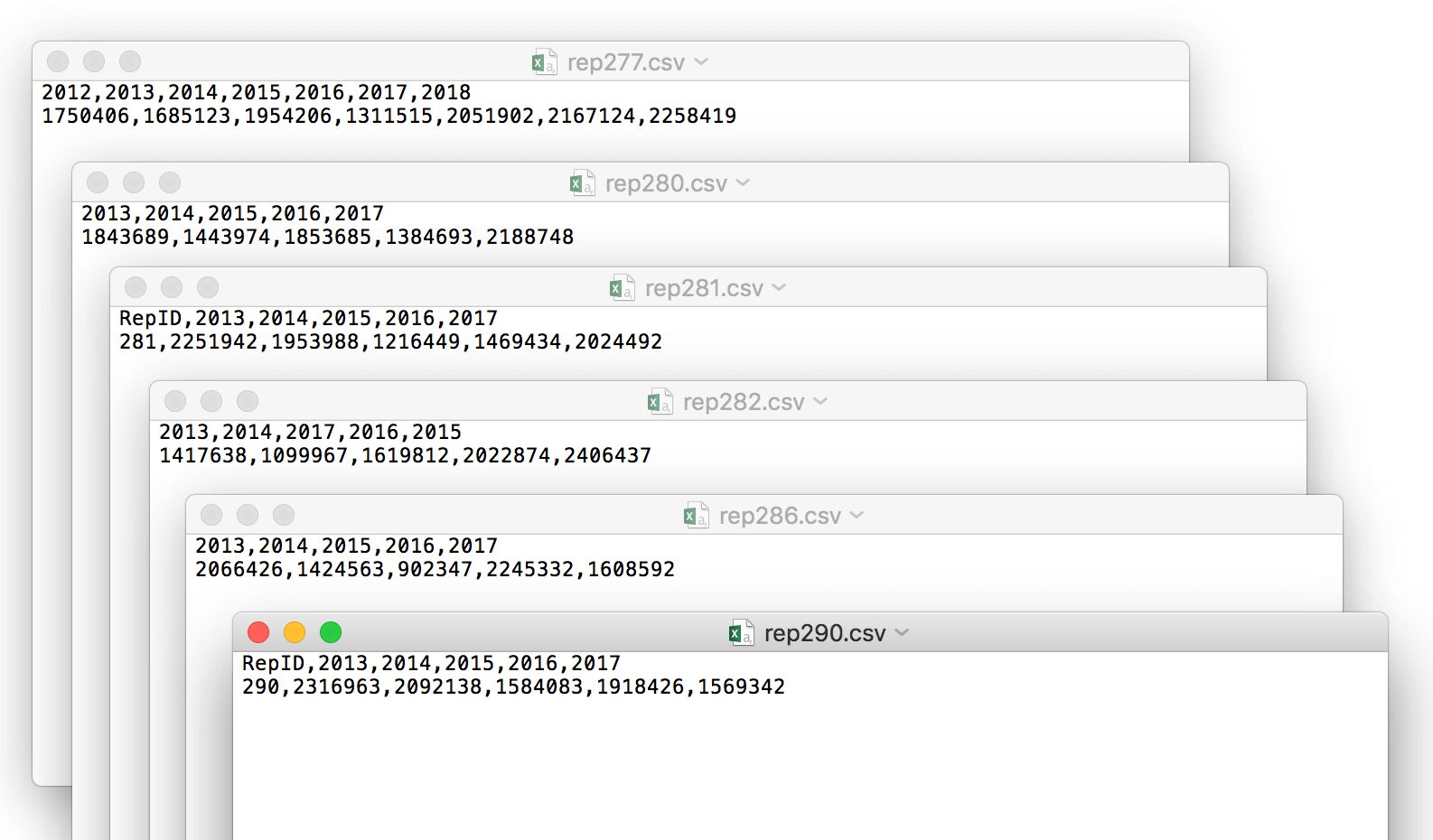
Each file includes the sales rep ID in the file name. This is the same ID returned by the RepID column of the df1 data set. Each file also contains the rep’s annual sales for five years (2013 through 2017), with some files containing additional information:
- Rep277.csv: Includes the five years, plus sales for 2012 and 2018.
- Rep280.csv: Includes only the five years.
- Rep281.csv: Includes the five years, plus the RepID column.
- Rep282.csv: Includes only the five years, but out of order.
- Rep286.csv: Includes only the five years.
- Rep290.csv: Includes the five years, plus the RepID column.
The .csv files are varied in order to try out different logic within the code. The goal here is to use only the .csv files that contain the five years of sales, regardless of the order of the columns or whether they include the RepID column. If the files include extra sales column or are in some other way inconsistent, they should be rejected, which in this case, would be the Rep277.csv file.
If you choose to create these files, try to follow the same logic used here, although you can use any numerical values for the sales totals. Once you have the .csv files in place, you’re ready to build the second data frame, as shown in the following example:
|
1 2 3 4 5 6 7 8 9 10 11 12 13 14 15 16 17 18 19 20 21 22 23 24 25 26 27 28 29 30 31 32 33 34 35 36 37 38 39 40 41 42 43 44 45 46 47 48 49 50 51 52 53 54 55 56 57 58 |
-- define Python script DECLARE @pscript NVARCHAR(MAX); SET @pscript = N' # import python modules import pandas as pd import glob # assign SQL Server dataset to the df1 variable df1 = InputDataSet df1["2012"] = df1["2012"].astype(int) # retrieve a list of the .csv files path = r"c:\\datafiles\\sales\\" files = glob.glob(path + "/*.csv") # define variables used to create a list for a data frame lst = [] vals1 = ["RepID", "2013", "2014", "2015", "2016", "2017"] vals2 = ["2013", "2014", "2015", "2016", "2017"] # open an output file for unusable .csv files outfile = open(path + "outfile.txt", "w") # define the generate_list function def generate_list(): if sorted(cols) == sorted(vals1): lst.append(df) elif sorted(cols) == sorted(vals2): start = file.find("rep") end = file.find(".csv") rep = file[start + 3:end] df.insert(0, "RepID", int(rep)) lst.append(df) else: start = file.find("rep") filename = file[start:] outfile.write(filename + "\n") # loop through each file in files to add data to list for file in files: df = pd.read_csv(file) cols = list(df.columns.values) generate_list() # close the output file outfile.close() # generate a data frame based on the data list df2 = pd.concat(lst, ignore_index=True) print(df2)'; -- define T-SQL query DECLARE @sqlscript NVARCHAR(MAX); SET @sqlscript = N' SELECT TOP(6) BusinessEntityID AS RepID, LastName + '', '' + FirstName AS FullName, CAST(SalesLastYear AS FLOAT) AS [2012] FROM Sales.vSalesPerson WHERE JobTitle = ''Sales Representative'' ORDER BY SalesLastYear DESC;'; -- run procedure, using Python script and T-SQL query EXEC sp_execute_external_script @language = N'Python', @script = @pscript, @input_data_1 = @sqlscript; GO |
The Python script in this example builds on the previous example by adding the code necessary to create the second data frame, starting with the following two import statements:
|
1 2 |
import pandas as pd import glob |
The pandas module includes the tools necessary to create and work with data frames. The glob module, which is new to this series, provides a simple way to retrieve a list of files, as shown in the following two lines of code, which have also been added to the script:
|
1 2 |
path = r"c:\\datafiles\\sales\\" files = glob.glob(path + "/*.csv") |
The first statement specifies the full path where the files are located and assigns it to the path variable. On my system, the files are saved to the c:\datafiles\sales folder, but you can use any folder. Just be sure to update the code as necessary. The second statement uses the glob function in the glob module to retrieve a list of the files in the sales folder and assign that list to the files variable.
The next step is to create a list object and save it to the lst variable:
|
1 |
lst = [] |
The variable will be used later in the script, within a for loop and then after the for loop. By declaring the variable now, you don’t have to be concerned about scope issues (although Python is very forgiving in this regard).
The next step is to assign a list of column names to the vals1 and vals2 variables:
|
1 2 |
vals1 = ["RepID", "2013", "2014", "2015", "2016", "2017"] vals2 = ["2013", "2014", "2015", "2016", "2017"] |
Later in the script, you’ll be comparing the variable values to the column names from the .csv files. In this way, only .csv files with matching column structures will be included in the data frame. All other files will be rejected and listed in the outfile.txt file. To write to the file, call the open function, providing the path and filename:
|
1 |
outfile = open(path + "outfile.txt", "w") |
In this case, I’ve used the path variable for specifying the file’s location, but you can target any location. Just be sure to include the w argument to tell Python that you’ll be writing to the file. The function will then create the file if it does not exist or overwrite the file if it does exist.
The output from open function is assigned to the outfile variable, which you’ll use later in the script to access the file.
The next step is to create a function named generate_list, which defines the logic necessary to process the .csv files:
|
1 2 3 4 5 6 7 8 9 10 11 12 13 |
def generate_list(): if sorted(cols) == sorted(vals1): lst.append(df) elif sorted(cols) == sorted(vals2): start = file.find("rep") end = file.find(".csv") rep = file[start + 3:end] df.insert(0, "RepID", int(rep)) lst.append(df) else: start = file.find("rep") filename = file[start:] outfile.write(filename + "\n") |
The function compares each file’s column names to the vals1 or vals2 variable and then takes the appropriate steps, depending on the results of the comparison. I’ve included the function primarily to demonstrate how you can use user-defined Python functions even if you’re working within the context of a SQL Server database. I’ll explain the function’s steps in more detail shortly. First, let’s look at the following for loop, which calls the function as its last step:
|
1 2 3 4 |
for file in files: df = pd.read_csv(file) cols = list(df.columns.values) generate_list() |
The for loop iterates through the list of files in the files variable. For each iteration, the individual file is assigned to the file variable. The first statement in the for loop uses the read_csv function from the pandas module to retrieve the data from the file specified in the file variable. The function saves the data to the df variable as a DataFrame object.
The second statement in the for loop retrieves a list of column names from the df data frame and saves the list to the cols variable. The third statement runs the generate_list function, which implements the following if…elif…else logic:
- If the cols values match the vals1 values, the df data frame is added to the lst object.
- If the cols values do not match the vals1 values, but match the vals2 values, the script takes several steps:
- Finds where “rep” is located in the filename and saves the location to start.
- Finds where “.csv” is located in the filename and saves the location to end.
- Uses start (plus 3) and end to extract the rep ID from the filename and save it to rep.
- Inserts the RepID column in the df data set, sets its value to rep, and converts the value to the int data type.
- Adds the df data frame the lst object.
- If the cols values do not match either the vals1 or vals2 values, the script takes the following steps:
- Finds where “rep” is located in the filename and saves the location to start.
- Uses start to extract the filename and save it to filename.
- Uses the write function on the outfile object to save the filename to the outfile.txt file, along with a line return.
Notice that the sorted function is used when calling the cols, vals1, and vals2 variables. This ensures that the values are being properly compared regardless of their original order.
When the for loop has completed, the lst object will contain each instance of the df data frame, unless the .csv file does not conform to either of the two conditions, in which case, the names of the unmatched files are saved to the outfile.txt file. The next step, then, is to close the file by calling the close function on the outfile variable:
|
1 |
outfile.close() |
Once you have the lst object populated with the individual data frames, you can concatenate them into a single data frame by using the concat function in the pandas module:
|
1 |
df2 = pd.concat(lst, ignore_index=True) |
The concat function specifies two parameters. The first parameter takes the lst variable as the data source. The second parameter, ignore_index, is set to True. This tells Python to disregard the individual indexes when generating the new data frame. The data frame is then assigned to the df2 variable. If you were to run a print statement against the new variable, you should see results similar to those shown in the following figure.
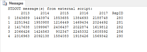
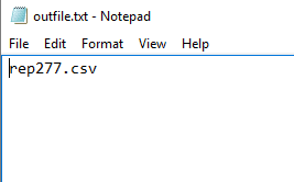
Notice that the df2 data frame contains data from five of the original files, even though two of those files include the RepID column and one includes columns that are out of order. The only file from the original set that was rejected is rep277.csv. The following figure shows how the rogue file is listed in the outfile.txt file.
Being able to redirect the filenames in this way allows you to easily identify which files do not conform to a particular structure. You could have tested for other logic as well, such as verifying whether the files contain extra rows or whether the filenames don’t conform to a particular structure. With Python, you can test for a wide variety of conditions, depending on your particular circumstances and requirements.
Merging two data frames
Now that you have your two data frames in place, you can merge them into a new data frame, which you can then modify even further, as shown in the following example:
|
1 2 3 4 5 6 7 8 9 10 11 12 13 14 15 16 17 18 19 20 21 22 23 24 25 26 27 28 29 30 31 32 33 34 35 36 37 38 39 40 41 42 43 44 45 46 47 48 49 50 51 52 53 54 55 56 57 58 59 60 61 62 |
-- define Python script DECLARE @pscript NVARCHAR(MAX); SET @pscript = N' # import python modules import pandas as pd import glob # assign SQL Server dataset to the df1 variable df1 = InputDataSet df1["2012"] = df1["2012"].astype(int) # retrieve a list of the .csv files path = r"c:\\datafiles\\sales\\" files = glob.glob(path + "/*.csv") # define variables used to create a list for a data frame lst = [] vals1 = ["RepID", "2013", "2014", "2015", "2016", "2017"] vals2 = ["2013", "2014", "2015", "2016", "2017"] # open an output file for unusable .csv files outfile = open(path + "outfile.txt", "w") # define the generate_list function def generate_list(): if sorted(cols) == sorted(vals1): lst.append(df) elif sorted(cols) == sorted(vals2): start = file.find("rep") end = file.find(".csv") rep = file[start + 3:end] df.insert(0, "RepID", int(rep)) lst.append(df) else: start = file.find("rep") filename = file[start:] outfile.write(filename + "\n") # loop through each file in files to add data to list for file in files: df = pd.read_csv(file) cols = list(df.columns.values) generate_list() # close the output file outfile.close() # generate a data frame based on the data list df2 = pd.concat(lst, ignore_index=True) # create the df_final data frame df_final = pd.merge(df1, df2, on="RepID") df_final.drop("RepID", axis=1, inplace=True) df_final.sort_values(by=["FullName"], inplace=True) print(df_final)'; -- define T-SQL query DECLARE @sqlscript NVARCHAR(MAX); SET @sqlscript = N' SELECT TOP(6) BusinessEntityID AS RepID, LastName + '', '' + FirstName AS FullName, CAST(SalesLastYear AS FLOAT) AS [2012] FROM Sales.vSalesPerson WHERE JobTitle = ''Sales Representative'' ORDER BY SalesLastYear DESC;'; -- run procedure, using Python script and T-SQL query EXEC sp_execute_external_script @language = N'Python', @script = @pscript, @input_data_1 = @sqlscript; GO |
As before, the script builds on the previous example by adding a few more lines of code. The first new statement merges the two data frames, based on the values in the RepID column.
|
1 |
df_final = pd.merge(df1, df2, on="RepID") |
To merge the data frames, you need only call the merge function from the pandas module, specifying the two data frames and matching column (RepID). The results are assigned to the df_final data frame.
Next, you can use the drop function available to the df_final object to remove the RepID column because it is not needed for the visualization:
|
1 |
df_final.drop("RepID", axis=1, inplace=True) |
When removing a column by name, you must include the axis parameter and set its value to 1. This tells Python to reference the column names rather than the column index labels. Also include the inplace parameter to ensure that the object is updated in place, rather than generating a new object.
The final statement added to the Python script sorts the df_final data frame based on the values in the FullName column:
|
1 |
df_final.sort_values(by=["FullName"], inplace=True) |
As with the drop function, be sure to include the inplace parameter when calling the sort_values function. You can then use a print statement to return the contents of the df_final data frame, which should give you results similar to those shown in the following figure.
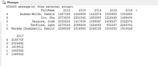
Notice that in the SSMS console, Python has wrapped the final column to the next row, which is indicated by the backslash to the right of the top row of column names. Even so, you can still see that the data set includes the names of the sales reps, along with their total sales for each of the six years.
Plotting the data frame
With the final data frame in place, you’re ready to create a bar chart the shows the annual sales for each sales rep:
|
1 2 3 4 5 6 7 8 9 10 11 12 13 14 15 16 17 18 19 20 21 22 23 24 25 26 27 28 29 30 31 32 33 34 35 36 37 38 39 40 41 42 43 44 45 46 47 48 49 50 51 52 53 54 55 56 57 58 59 60 61 62 63 64 65 66 67 68 69 70 71 72 73 74 75 76 77 78 79 80 81 |
-- define Python script DECLARE @pscript NVARCHAR(MAX); SET @pscript = N' # import python modules import matplotlib matplotlib.use("PDF") import matplotlib.pyplot as plt import pandas as pd import glob # assign SQL Server dataset to the df1 variable df1 = InputDataSet df1["2012"] = df1["2012"].astype(int) # retrieve a list of the .csv files path = r"c:\\datafiles\\sales\\" files = glob.glob(path + "/*.csv") # define variables used to create a list for a data frame lst = [] vals1 = ["RepID", "2013", "2014", "2015", "2016", "2017"] vals2 = ["2013", "2014", "2015", "2016", "2017"] # open an output file for unusable .csv files outfile = open(path + "outfile.txt", "w") # define the generate_list function def generate_list(): if sorted(cols) == sorted(vals1): lst.append(df) elif sorted(cols) == sorted(vals2): start = file.find("rep") end = file.find(".csv") rep = file[start + 3:end] df.insert(0, "RepID", int(rep)) lst.append(df) else: start = file.find("rep") filename = file[start:] outfile.write(filename + "\n") # loop through each file in files to add data to list for file in files: df = pd.read_csv(file) cols = list(df.columns.values) generate_list() # close the output file outfile.close() # generate a data frame based on the data list df2 = pd.concat(lst, ignore_index=True) # create the df_final data frame df_final = pd.merge(df1, df2, on="RepID") df_final.drop("RepID", axis=1, inplace=True) df_final.sort_values(by=["FullName"], inplace=True) # create a bar chart object pt = df_final.plot.bar(x="FullName", cmap="copper") # configure the title, legend, and grid pt.set_title(label="Annual Sales by Sales Rep", y=1.04, fontsize=14) pt.legend(loc=7, bbox_to_anchor=(1.2, .8)) pt.grid(color="slategray", alpha=.5, linestyle="dotted", linewidth=.5) # configure the Y-axis labels pt.set_ylabel("Total Sales", labelpad=20, fontsize=12) pt.get_yaxis().set_major_formatter(matplotlib.ticker.FuncFormatter (lambda x, p: format(int(x), ","))) # configure the X-axis labels pt.xaxis.label.set_visible(False) pt.set_xticklabels(labels=df_final["FullName"], rotation=45, horizontalalignment="right") # save the bar chart to a PDF file plt.savefig(path + "AnnualSales.pdf", bbox_inches="tight", pad_inches=.5)'; -- define T-SQL query DECLARE @sqlscript NVARCHAR(MAX); SET @sqlscript = N' SELECT TOP(6) BusinessEntityID AS RepID, LastName + '', '' + FirstName AS FullName, CAST(SalesLastYear AS FLOAT) AS [2012] FROM Sales.vSalesPerson WHERE JobTitle = ''Sales Representative'' ORDER BY SalesLastYear DESC;'; -- run procedure, using Python script and T-SQL query EXEC sp_execute_external_script @language = N'Python', @script = @pscript, @input_data_1 = @sqlscript; GO |
Most of the code related to the visualization was covered in third article, so we won’t dig into it too deeply. As you’ll recall, you must include the following import and use statements:
|
1 2 3 |
import matplotlib matplotlib.use("PDF") import matplotlib.pyplot as plt |
The matplotlib module provides a set of tools for generating different types of visualizations and saving them to files. The first statement imports the module, the second statement uses the module to set the backend to PDF, and the third statement imports the pyplot plotting framework. The three statements make it possible to output the visualization it to a .pdf file.
The next step is to define the actual bar chart, calling the plot.bar function on the df_final data frame:
|
1 |
pt = df_final.plot.bar(x="FullName", cmap="copper") |
For this visualization, the plot.bar function takes only two parameters. The first specifies that the FullName column should be used for the chart’s X-axis. The second parameter, cmap, sets the chart’s colormap. A colormap is essentially a monochromatic color palette made up of different shades of a common color. When creating a chart, you can choose from a number of different colormaps. In this example, I’ve selected copper, but feel free to try different ones. (You can learn more about colormaps at https://matplotlib.org/tutorials/colors/colormaps.html.)
The chart generated by the plot.bar function is assigned to the pt variable. Most of the remaining Python code uses the variable to access the chart’s properties in order to control how the chart is rendered. From there, the chart is saved to the AnnualSales.pdf file. Again, refer back to the third article if you have any questions about these settings.
That’s all there to creating the bar chart. If you followed along with this example, your Python script should produce a chart similar to the one shown in the following figure.
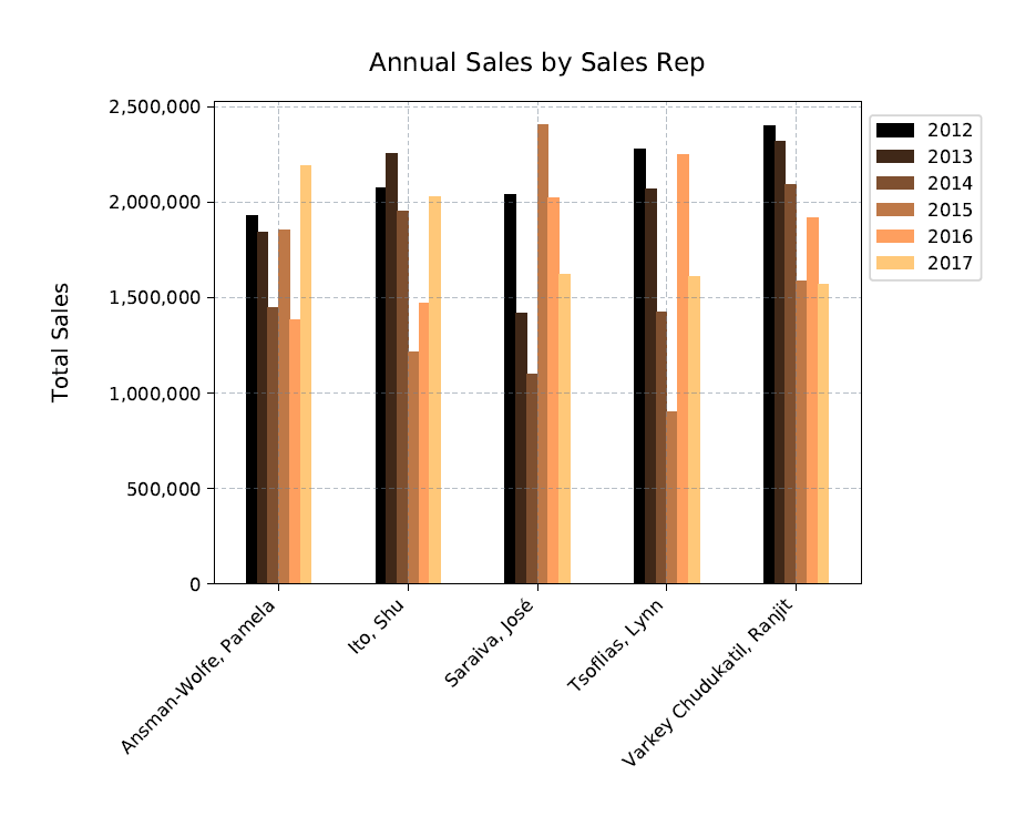
What’s interesting about all this is how the plot.bar function intuitively handles the data, in this case, grouping together the sales for each rep and then applying the copper colormap to each group. Notice, too, that the legend automatically picks up the column names, while color-coding the keys to match the bars in each group.
Working with Python in SQL Server
In this and the previous articles in this series, we’ve covered a number of aspects of working with data frames, as they relate to both analytics and visualizations. Of course, there’s much more you can do with any of these. And there’s plenty more you can do with Python and MLS in general. The better you understand how to work with Python scripts in SQL Server, the more powerful a tool you have for analyzing and visualizing data.