The series so far:

1. SQL Server Graph Databases - Part 1: Introduction
2. SQL Server Graph Databases - Part 2: Querying Data in a Graph Database
3. SQL Server Graph Databases - Part 3: Modifying Data in a Graph Database
4. SQL Server Graph Databases - Part 4: Working with hierarchical data in a graph database
5. SQL Server Graph Databases - Part 5: Importing Relational Data into a Graph Database

This first three articles in this series focused on using SQL Server graph databases to work with data sets that contained relationships not easily handled in a typical relational structure, the types of relationships you might find in a social network site or product recommendation engine. One of the topics that the articles touched upon was how to work with hierarchical data and their relationships, as they applied to the FishGraph database used in the examples.

This article digs deeper into the topic of hierarchies, particularly those that contain more complex relationships than what you saw in the examples. The article first provides an overview of how to create and populate the tables necessary to support a hierarchy and then focuses on how to query hierarchical data that contains multiple types of relationships.

Limitations of the HierarchyID Data Type

Working with hierarchical data is certainly not new in SQL Server. Since the product’s early days, you could represent a hierarchical structure by including a foreign key in a table that pointed to the primary key in the same table. In this way, you were able to represent the parent-child relationships that existed within the data set.

Since the release of SQL Server 2008, you’ve been able to use the hierarchyid data type to represent a record’s hierarchical position by defining values that reflect the relationships between a table’s rows. For example, the data type makes it possible to represent how employees are organized within a company’s hierarchical structure, such as the one shown in the following figure.

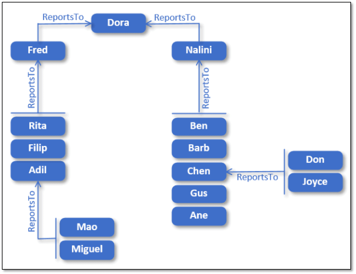
Although this is a very simple example, it demonstrates the types of relationships that typically make up a basic hierarchy:

• Dora sits at the top of the hierarchy.
• Fred and Nalini report to Dora.
• Rita, Filip, and Adil report to Fred.
• Ben, Barb, Chen, Gus, and Ane report to Nalini.
• Mao and Miguel report to Adil.
• Don and Joyce report to Chen.

As with the above figure, a hierarchy is often represented as an inverted tree structure in which all branches lead to a common root, in this case, Dora.

Unfortunately, not all hierarchies are this simple. For example, an employee might work part time in two positions, which means reporting to two different managers. Or an employee might report to one manager but actually work for another, that is, the employee is managed by someone different from whom the employee reports to.

A hierarchy that reflects real-world situations will likely be a lot less straightforward that the one shown in the previous figure. Even an example as simple as this one can end up being a lot more complex after adding a few exceptions, as shown in the following figure.

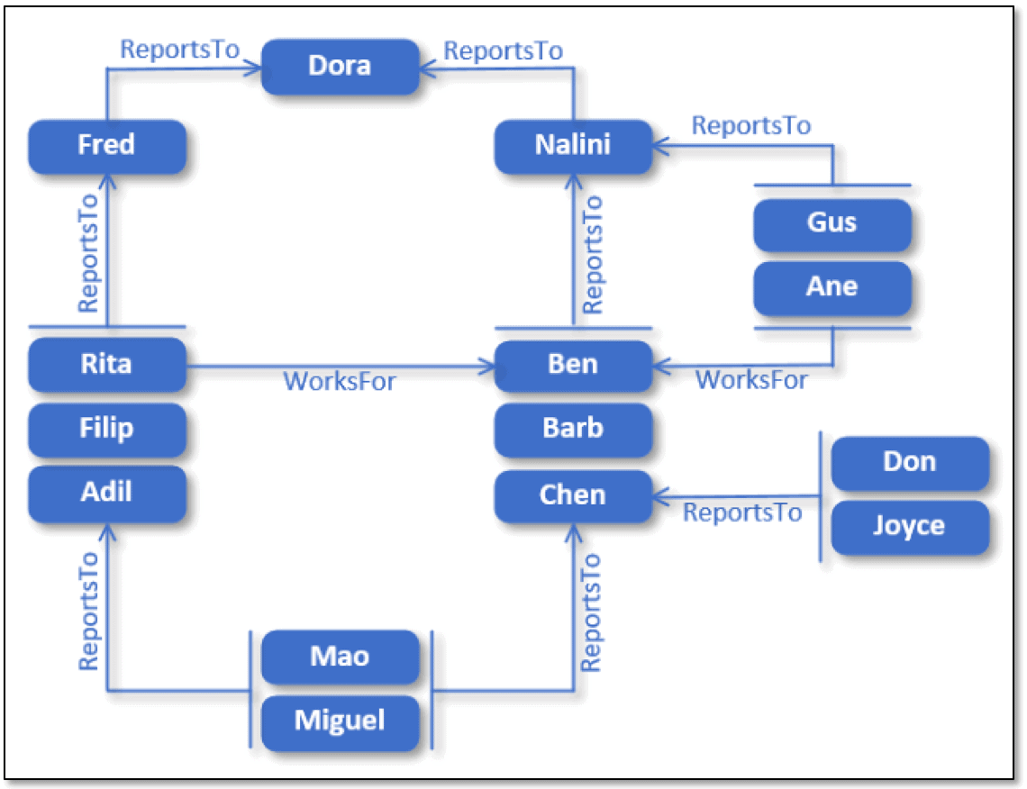
Although many of the basic relationships are the same, the hierarchy now includes people who report to more than one manager or who report to one manager but work for another:

• Dora sits at the top of the hierarchy.
• Fred and Nalini report to Dora.
• Rita, Filip, and Adil report to Fred, but Rita works for Ben.
• Ben, Barb, Chen, Gus, and Ane report to Nalini, but Gus and Ane work for Ben.
• Mao and Miguel report to both Adil and Chen, working half-time in each position.
• Don and Joyce report to Chen.

The hierarchyid data type is not equipped to handle anything that does not fit neatly into a basic structure. And even if the hierarchy does fit this model, too many levels can still be difficult to manipulate and maneuver. Graph databases, on the other hand, are made for more complex hierarchies, regardless of the number of levels or types of relationships, making it easier to accommodate the hierarchy, rather than trying to force the hierarchy into a relational structure.

Defining the Graph Tables

The previous articles in this series used the FishGraph database to demonstrate various graph concepts. This article also uses the database, but only to add tables based on the employee hierarchy shown in the above figure. The tables are unrelated to the existing FishGraph tables, so if you’re trying out these examples, you can use any database you want. That said, including the tables in the FishGraph database opens up the potential for creating relationships between the new and original tables with very little effort, should you be inclined to do so.

To implement the employee hierarchy, you need to create and populate three tables, one node table to store the list of employees and two edge tables to store the reports to and works for relationships defined between those nodes.

The first table, FishEmployees, is a node table that contains the ID and first name of each employee, along with the auto-defined $node_id column. The following T-SQL script creates and populates that table:

We won’t spend too much time on how to create and populate graph tables because these concepts are covered extensively in the first article. The main point to keep in mind is that you must include the AS NODE clause when creating a node table and the AS EDGE clause when creating an edge table. The database engine will then add the necessary auto-defined columns.

The next table is ReportsTo, an edge table that records each reports to relationship between employees. You can create and populate the table without including any user-defined columns, as shown in the following T-SQL script:

Each INSERT statement retrieves the $node_id values from the FishEmployees table in order to provide the relationship’s originating and terminating nodes (the $from_id and $to_id values, respectively). You can take a similar approach for the third table, FishEmployees, which records each works for relationship between employees:

That’s all there is to defining the employee hierarchy shown in the above figure. Although this is a simple example, it demonstrates many of the concepts associated with building a more complex hierarchy that contains numerous levels and multiple types of relationships. For a single hierarchy, you need a node table for the primary entities and an edge table for each type of relationship within that hierarchy. In this way, you can define as many types of relationships as necessary and define multiple relationships within a single type that share the same child node but different parent nodes. (If you have any questions about creating or populating graph tables, refer back to the first article in this series.)

Returning employee data

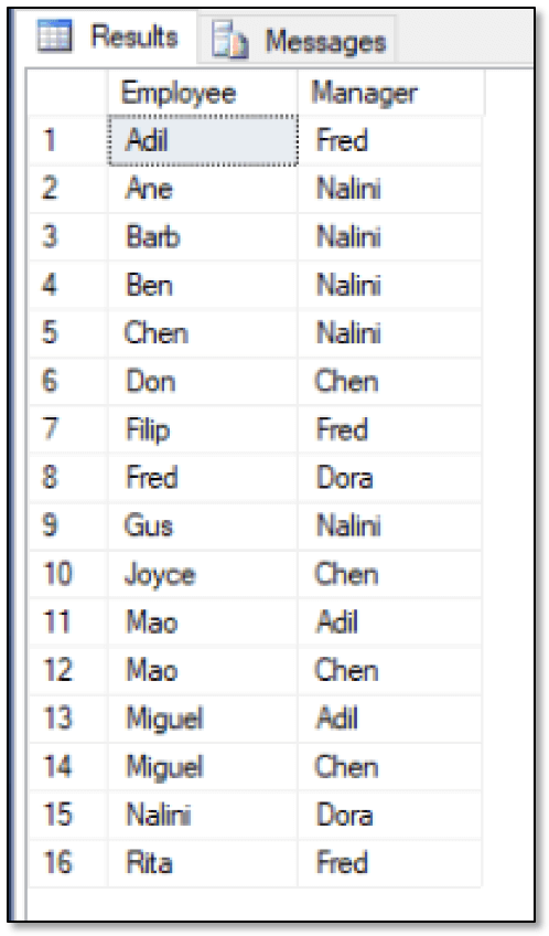
Querying graph tables that support a hierarchy is just like querying any tables in a graph database, something we covered in detail in the second article. For example, to view all the reports to relationships in the employee hierarchy, you can run the following SELECT statement:

The statement uses the MATCH function to return a list of employees and the people they report to. Because the originating and terminating nodes reside in the same table, you must specify the table twice in the FROM clause, providing a different alias for each instance. You can then use those aliases in the MATCH clause, along with the name of the edge table, to specify the relationship employee 1 reports to employee 2. The SELECT statement returns the results shown in the following figure.

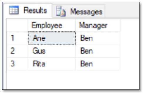
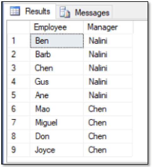
You can take a similar approach to view all the works for relationships:

This time the query returns the results shown in the next figure, which indicate that three employees work for Ben.

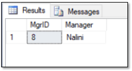
So far, this is all fairly basic. The MATCH function makes it easy to find the relationships defined between nodes, whether those nodes are in the same table or in different tables. To return more specific information, you can modify the WHERE clause to include additional conditions. For example, the following SELECT statement returns the employee ID and name of the manager that Barb reports to:

When adding this type of condition to the WHERE clause, be sure to reference the correct node. In this case, you should use the emp1 table alias, rather than emp2, because you need to reference the originating node, not the terminating one. The SELECT statement returns the results shown in the following figure.

As you can see, retrieving the name of an employee’s manager is fairly straightforward. However, not all queries are this simple. For example, if you want to know which employees report to more than one manager, you must take a different approach. One solution is to create a common table expression (CTE) that retrieves the node IDs of the employees with more than one manager. You can then use the CTE as one of the conditions in the WHERE clause of the outer SELECT statement to return those relationships:

The CTE retrieves the $from_id values from the ReportsTo table, using the GROUP BY and HAVING clauses to return only those IDs that include multiple instances. The WHERE clause in the outer SELECT statement then uses an IN expression to compare the $from_id values to those returned by the CTE, giving us the results shown in the following figure.

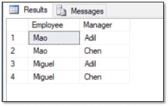
As you can see, the results show the two employees, Mao and Miguel, and their managers, Adil and Chen. Now suppose you want to view the name of employees who report to one manager, but work for another manager. In this case, you don’t need to use a CTE because the MATCH function can give you the information you need:

As you’ll recall from the second article, you can point the MATCH relationships in either direction. In this case, the function includes two relationships with both of them originating with the emp1 node. The first relationship is a reports to relationship that terminates with the emp2 node. The second relationship is a works for relationship that terminates with the emp3 node. As a result, the SELECT statement will return only those rows in which an employee both reports to an individual and works for an individual, as shown in the following results.

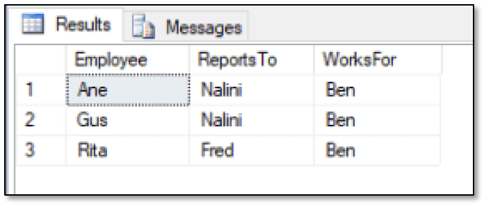
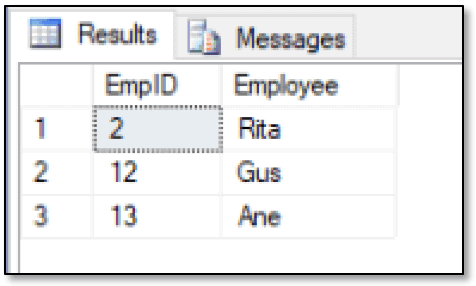
As expected, only three employees fit this scenario. If you instead want to view only those employees who work for Ben, you can simplify your query even further:

In this case, the SELECT statement returns the ID and name of each employee who works for Ben. To get this data, you need include only a simple MATCH relationship and a second WHERE clause condition limiting the relationships to those that terminate with Ben, giving you the following results.

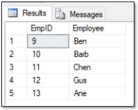
You can do something similar to find the employees who report to Nalini:

Now the SELECT statement returns the results shown in the next figure.

The flexibility of the MATCH clause, along with the ability to use CTEs when necessary, allows you to return different types of data sets from a hierarchy. It might take some trial-and-error to get it right, but eventually you should be able to retrieve the results you want. In some cases, however, the MATCH clause—with or without a CTE—will not return the data you need, and you’ll have to look to other strategies.

Bumping up against graph limitations

Because the graph features are so new to SQL Server, it’s not surprising that they have several limitations. For example, you cannot use the MATCH function on derived tables, which means you cannot use the function in the recursive member of a CTE. Graph databases also don’t support transitive closure—the ability to search recursively through graph tables beyond the first level.

To get around these limitations, you must use more traditional T-SQL. For example, you can retrieve a list of employees who report directly or indirectly to a specific manager by creating a recursive CTE, without using the MATCH function:

The CTE uses the UNION ALL operator to recurse through the employees and determine who reports to Nalini. The first SELECT statement establishes the form of the result set, based on the Nalini record, and provides the starting point for recursing through the data. The Manager column acts as a placeholder for the corresponding column returned by the second SELECT statement, which joins the FishEmployees and ReportsTo tables to the emp CTE to provide the recursive element. The outer SELECT statement then retrieves the data from the CTE, filtering out the Nalini record, as shown in the following results.

As you can see, the first five employees report directly to Nalini, and the remaining four employees report directly to Chen, who is one of the five who reports to Nalini.

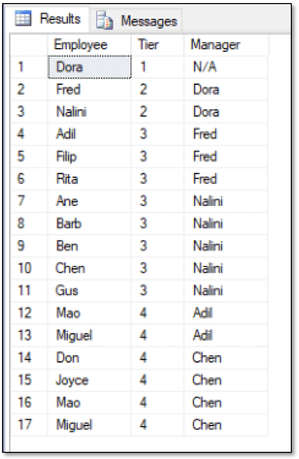
You can also use a recursive CTE to return a list of employees and the levels, or tiers, in which those employees are positioned within the hierarchy:

This time around, the first SELECT statement in the CTE returns a row for Dora, who sits at the top of the hierarchy. The statement also returns an additional column, Tier, which is assigned a value of 1 to represent the first tier. The second SELECT statement then adds 1 to the Tier value with each recursion. Most of the other T-SQL elements are the same as in the preceding example, except that now the results look much different, as shown in the following figure.

You can also use this statement structure to return a single tier of employees, in this case, the third tier:

The most important difference here, when compared to the preceding example, is that the WHERE clause now specifies which tier to return, giving you the results shown in the following figure.

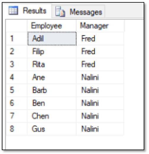
As you can see, only the employees in the third tier are included in the results, along with the names of their managers, Fred and Nalini. You can, of course, come up with other ways to slice and dice the data, depending the type of information you’re trying to retrieve.

Viewing a Hierarchy

There might be times when you want to get a less ‘recursive’ view of the data so you can see everyone in the management chain under a specific manager in a single view. To demonstrate how to do this, you can take your cue from Phil Factor’s informative article SQL Server Closure Tables, where he describes how to use closure tables to represent hierarchies.

To make his approach work on the FishEmployees hierarchy, you should create a function that retrieves the ID and name of each employee who reports to a specific manager. The function should also assign the tier level to each employee, relative to that manager, as shown in the following example:

The function takes a single parameter, the manager’s employee ID, and returns all the employees who report directly or indirectly to that manager. You will run the function for each employee so you have a mapping of the entire employee chain, as you’ll see shortly.

The challenge with this approach is that it does not handle employees who report to more than one manager, as is the case with the FishEmployees hierarchy. For this example, you can run the following two DELETE statements to remove the conflict, keeping in mind that ultimately you would have to include the logic necessary to handle this situation:

Next, you should create a temporary table, retrieve the first employee ID from the FishEmployees table, and then run a WHILE loop that uses the function to populate the table:

The WHILE loop runs the GetEmployees function for each employee ID until there is none left, adding the returned data to the #temp table with each iteration.

The #temp table essentially acts as the type of closer table described by Phil Factor. I’ve included the employee and manager names in the results as an easy way to verify the data, but they’re not necessary to the final product. One thing to note about this process is that the tier levels assigned to each employee are relative to the specific employee being called when the function runs, rather than applying universally across the entire hierarchy. This is essential to creating a proper closure table.

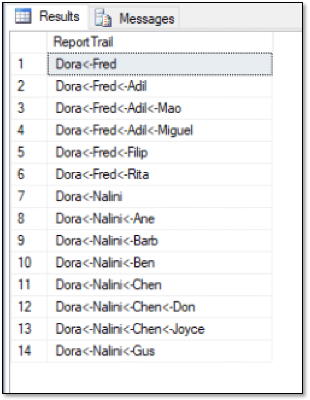
Once the #temp table is populated with the employee data, you can run a SELECT statement that retrieves the management chain by using a combination of self-joins and careful sorting:

The query creates the self-joins within a subquery, specifying several WHERE conditions to limit the results. The subquery uses the FOR XML output type, along with the value function available to the XML data type, to get the data in a linear format. The outer WHERE clause applies additional filters, along with another ORDER BY clause, providing the results shown in the following figure.

For more information about how the closure table and query work, refer to the Phil Factor article, which goes into far more detail about the different ways you can use closure tables with hierarchical data.

Working with hierarchical relationships

SQL Server graph databases have a number of limitations, especially when it comes to the types of advanced querying available to more mature graph technologies. As a result, you might find yourself having to revert to the sort of workarounds demonstrated in the last section. However, because the SQL Server graph database features are based on traditional relational tables, you can usually figure out some way to get the data you need, even if that data lies within a complex hierarchical structure. You might have to work a bit to return the desired results, but eventually you should be able to get at the correct information.