Power BI Desktop provides a robust adjunct to the Power BI services by offering access to a wider range of data sources and transformations, in addition to its offline capabilities. At the heart of Power BI Desktop is the Power Query Formula Language (PQFL), a dynamically typed, case-sensitive functional language for creating mashup queries, similar to the F# language. Although Power BI Desktop has a number of UI features for simplifying transformations, PQFL underpins those transformations, and the better you understand the language, the more you can take advantage of the capabilities inherent in Power BI Desktop.

Formerly known as M, PQFL has its roots in Power Query for Excel, and as such, much of the information you find about the language is specific to Excel. Although this will likely change as Power BI Desktop catches on, currently it can be difficult to find examples specific to Power BI Desktop that will help you resolve a particular issue. That said, PQFL follows a very specific formula that is uniform enough to make it relatively painless, at least in some cases, to come up with solutions on your own, as long as you know the basics.

In this article, I introduce you to PQFL so you can see for yourself how to use the language to create mashup queries from scratch. If you’re not familiar with Power BI Desktop, I suggest you first review my article Working with SQL Server data in Power BI Desktop, which provides details on how to get started using the application to retrieve and transform data.

Each transformed data set in Power BI Desktop is essentially a PQFL query that retrieves data from a source and modifies the data in various ways. To create a PQFL query, you start with a let expression that contains a series of expression steps.

Each step is in essence its own expression that assigns a value to a variable, based on a combination of functions, operators, and value types. The value types can include simple primitive scalar values such as numbers or strings, or include objects such as lists, records, or tables. The variable can then be used in one or more subsequent expression steps, which themselves define additional variables. This will all become clearer as we work through a few examples.

For this article, we’ll be retrieving data from a SQL Server database, so we’ll be restricting ourselves primarily to table objects and primitive values; however, the concepts we cover apply to all object types. To demonstrate these concepts, I created a set of examples based on data from the AdventureWorks2014 database on a local instance of SQL Server 2014. Each example builds in the previous one in order to demonstrate how to create a PQFL query one expression step at a time. With that in mind, let’s get started.

Retrieving data from SQL Server

In Power BI Desktop, you can create a PQFL query without first connecting to a data source. Instead, you define the connection within the let expression, as the first expression step. To begin, open Query Editor and take the following steps:

1. Click the New Source button on the Home ribbon, and then click Blank Query. A new query is added to the Queries pane (named Query1, by default).
2. In the Properties section of the Query Settings pane, type a new name for the query. I used RepSales because we’re going to create a data set based on the annual sales of the Adventure Works sales reps.
3. In the Queries pane, right-click the new query, and then click Advanced Editor.

The last step launches the advanced editor, with the start of a let expression already defined, as shown in the following figure.

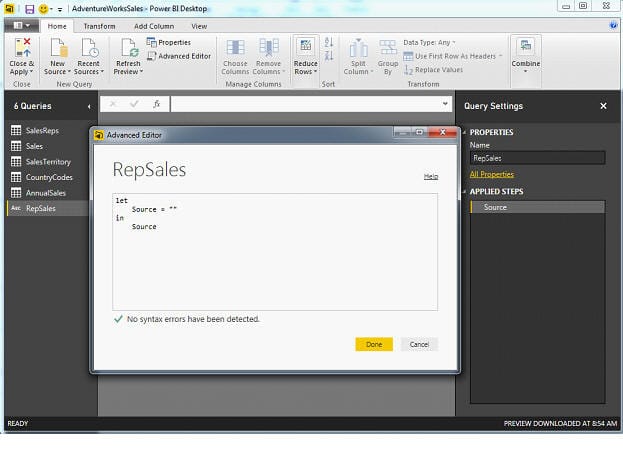
The let expression includes two parts, the let statement and the in statement. The let statement defines the expression steps, and the in statement specifies variable, which determines what data the query returns.

The first expression step in the let statement defines the Source variable as an empty string. Ultimately, the variable will be used to identify the initial data source.

You don’t need to stick with naming the variable Source. You can use just about any name you want within reason. PQFL even supports variable names that contain spaces, but then you must enclose the variable name in quotes and precede it with a hash mark, a rather messy coding convention that I try to avoid. Whatever you name your variables, keep in mind that PQFL is a case-sensitive language, which applies to all elements.

The first step, then, is to change the variable definition to something other than an empty string. For that, we can turn to one of the many PQFL functions available to the various types of objects and primitive values. Because we will be retrieving data from a SQL Server database, we’ll use the Sql.Database function to specify the SQL Server instance, database, and a T-SQL query, as shown in the following let expression:

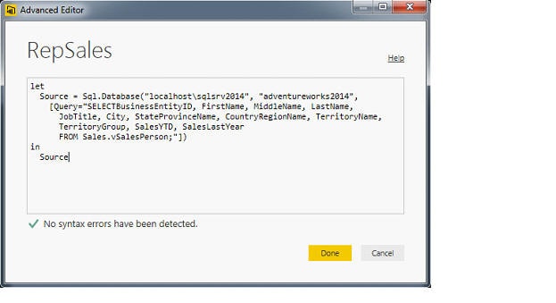
As you can see, the Source definition uses the Sql.Database function to call the AdventureWorks2014 database on a named SQL Server instance (localhost\sqlsrv2014). The Query option, which is enclosed in brackets, defines a straightforward T-SQL query that retrieves data from the Sales.vSalesPerson view. Of course, we can make our T-SQL query far more complex, or we can keep it simple and do the work in our let expression, which is what we’ll do here.

That’s all there is to defining the initial data source. The following figure show what the Advanced Editor window should look like after we’ve updated the Source definition.

Before we continue, it’s worth pointing out that the advanced editor in Power BI Desktop is anything but advanced. It is barely a step above Notepad, providing only a rudimentary syntax checker. If it does find a problem, the checker often fails to point to the correct part of the syntax, or worse still, the checker misses the error altogether, and it’s not until you run your query that you discover something is wrong.

You also cannot save your changes as you go along within the advanced editor. If the syntax checker fails to find an error, and running the code crashes the system, you will lose all your changes, which has happened to me. One way to protect yourself again this particular scenario is to copy your work over to Notepad or some other text editor as you’re working so you don’t risk losing what you’re doing. You should also run your query whenever you add or modify an expression step. If the query runs successfully, you can apply and save your work.

The advanced editor is not particularly conducive to trial-and-error development. Whenever you want to check the results of a code change, you must exit the environment to run the query (and save it) and then re-launch the editor to continue, usually having to resize the window with each cycle. With luck, Microsoft will improve this feature at some point in the future, if enough of us whine about it.

Now that you’ve been warned, we can move forward. If you’re satisfied with your let expression as it stands, click Done to close the advanced editor and run the query. Your results should now look similar to the Query Editor window shown in the following figure.

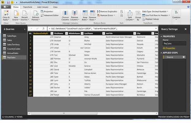
If you’ve gotten this far, you have now successfully retrieved the data from SQL Server and you can start transforming it.

Filtering rows

Often, when you’re developing your let expression, you will use the variable you define in one step as part of the expression in the next step. In this way, you create your query as well defined and delineated steps that build on each other.

To demonstrate how this works, we’ll filter out all rows whose TerritoryName value is null. The idea is to remove all managers from our list so we end up with only the sales reps. We can instead filter the data based on the JobTitle column, retrieving only those rows that contain the Sales Representative value. I went with the nullability factor because strings are easier to mess up when you’re typing, but you can do whatever works best in your particular circumstances. Given that this is just an example, I went for the low-hanging fruit.

To filter the data, we’ll use the Table.SelectRows function. As you might have noticed with the Sql.Database function, PQFL functions are usually specified as two-part names. The first part is the object type, and the second is the actual function name. For the Sql.Database function, the object type is Sql, and for the Table.SelectRows function, the object type is Table.

The Table object type supports a wide range of functions, as do all the object types. You can find a comprehensive list of the PQFL functions in the Power Query Formula Reference. In the meantime, let’s return to our let expression and add a second variable definition, which we’ll name SalesRep:

To add a new variable definition, we add a comma after the first expression step and start the new definition with the variable name, as we did with the first one. There is no need to specifically declare or type variables in PQFL. The typing occurs as part of the variable definition.

In this case, we’re creating a table object, as determined by the the Table.SelectRows function, which returns a table object, just like the Sql.Database function. The Table.SelectRows function takes two arguments. The first is the input table, the Source variable, and the second is the expression that determines which rows to filter out. In this case, the expression uses the each function to iterate through the rows. For each row, the TerritoryName column must not be null.

That’s all there is to filtering rows, but also notice that the in statement now calls the SalesRep variable, rather than Source. The SalesRep variable contains the transformed data, which is the data we want to return. Generally, you should define your if statement to call the last variable defined in the let statement.

Creating a custom column

Next we’ll create a custom column named FullName that concatenates each sales rep name. However, we’ll need to include conditional logic in our variable definition to account for those reps with a null MiddleName value. For that, we’ll include an if expression in the variable definition, as shown in the following let statement:

We start by adding the RepName variable, following by the definition. The definition uses the the Table.AddColumn function, which takes three arguments. The first argument specifies the table source, SalesRep, and the second argument specifies the name of the new column, FullName.

The third argument is the column expression that does all the work. The expression begins with the each function, a special function used to iterate through a collection of data. This is followed an the if expression, which defines the conditional logic needed to know how to concatenate the names. If the MiddleName value is not null, the FirstName, MiddleName, and LastName values are concatenated, with spaces in between. Otherwise, only the FirstName and LastName values are concatenated, again, with a space.

Although this is only a simple example of using an if expression, it demonstrates what a powerful tool you have available for transforming your data. You can create a data set that accounts for different types of values. Notice also that this time our in statement calls the RepName variable to ensure that our let expression returns the fully transformed data.

Removing columns

Now let’s do a few more transformations, starting with removing the columns we no longer need: FirstName, MiddleName, LastName, and JobTitle. Because the expression steps build on each other, we can remove these columns without affecting previous operations. In other words, the most recent variable, RepName, represents our data set’s current reality, allowing us to act on the variable however we need to without looking back.

To remove the columns, we’ll create a variable named RemoveCols and invoke the Table.RemoveColumns function, as shown in the following example:

The Table.RemoveColumns function takes only two arguments, the table source, RepName, and the list of columns to delete. For such a list, the column names must be enclosed in quotes and separated by commas, and the entire list must be enclosed in curly braces.

Renaming columns

At this point, you should have a good sense of how the expression steps build on each other as you continue to apply transformations to your data. We can take this same approach to rename columns:

This time around, we create a variable named RenameCols and include in the definition the the Table.RenameColumns function, which takes two arguments. The first argument, as you’ve seen with other functions, identifies our source table, RemoveCols, and the second argument provides a list of columns to rename. Each element in the list specifies the column’s original name and its new name, with the names enclosed in their own set of curly braces. For example, we’re changing the name of the BusinessEntityID column to RepID, and we’re change the name of the StateProvinceName column to StateProvince.

Rounding numerical data

We can also add expression steps that round the numerical columns, SalesYTD and SalesLastYear, but we have to take a slightly different approach from the previous two examples. We’ll still call a Table function, Table.TransformColumns, which also takes two arguments, but the second argument includes a couple other functions, as shown in the following let expression:

I’ve created two expression steps to more easily explain the components, but we could have instead used one step. The first step defines the RoundSalesYTD variable. The Table.TransformColumns function takes two arguments: the source table, RenameCols, and the transform operation. The transform operation is made up of three components. The name of the target column, SalesYTD, an expression that performs the actual transformation, and the return type, number.

The transformation expression starts with the each function, followed by the Number.Round function, which does the actually rounding. This function also takes two arguments: the value to round and the number of decimal points to apply. In this case, the value to round is an underscore (_), which simply represents the column’s current value, and the 0 indicates that the outputted value should contain no decimal points.

The next expression step, which defines the RoundSalesLastYear variable works this same way, just with a different column. If you want to instead turn these two steps into one, you can do something like the following:

For now, however, we’ll keep the expression steps separate and move on to our next transformation.

Reordering columns

You might find that you don’t like the order of the columns in a data set, in which case you can use the Table.ReorderColumns function, which also takes only two arguments: the source table, RoundSalesLastYear, and the list of columns in the order you want them:

All very straightforward. The only trick is to enclose the list of columns in curly braces, separate the column names with commas, and enclose each column name in quotes.

Building on multiple variables

Now let’s look at one final transformation in which we add another custom column. This time, however, we’re going to use a series of embedded if expressions to set the value. We’re also going to do something else-introduce a second variable to add to the mix. Let’s start by looking at the updated let expression:

The new section of code starts with a comment, as indicated by the double forward slashes. I threw this in just to show you that PQFL supports one-line comments like this and multi-line comments that follow T-SQL conventions (/* and */).

Next, we define a variable whose sole purpose is to capture the average amount of sales from the SalesLastYear column. To get the average, we add the LastYearAvg variable and start the definition with the List.Average function. We’re using a List function because the Table object doesn’t support an Average function. The List.Average function takes one argument, which itself calls the Table.Column function. The Table.Column function merely retrieves the SalesLastYear values from the ReorderCols table so that the List.Average function can calculate the average of those values. On my system, the average comes to 1691854.5446.

We can now use the LastYearAvg variable in subsequent expression steps as part of our calculations. The next step, then, defines the SalesStatus variable, which uses the Table.AddColumn function to insert a custom column into the data set. Notice that the function’s first argument refers to the ReorderCols variable, not the LastYearAvg variable. We want to return to our main data set and work from there.

The SalesStatus definition is similar to the RepName definition, except that the embedded if expressions are somewhat more involved with SalesStatus. What we’re trying to do here is assign values to the new column based on how each SalesYTD value compares to the average sales for the previous year, as determined by the LastYearAvg variable. (PQFL doesn’t support anything comparable to a CASE expression.) Essentially, we’re just adding an if expression to the else clause of the previous if expression.

The logic in these if expressions is fairly straightforward. A value is assigned to the column based on how it evaluates against last year’s average. Your final data set should now look similar to what’s shown in the following figure.

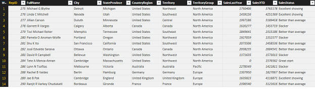
The main point to take out of this last transformation is that you don’t have to stick strictly to the formula of defining one variable after the other and using that variable in the next step. The steps must still proceed lineally, so you have to account for that, but you also have room to play.

Creating visualizations

Once you have applied and saved your data set, you can use it just like any other data set. For example, I created the following visualization based on the FullName, SalesYTD, and SalesStatus columns.

A simple, yet telling visualization, which is exactly what a visualization is supposed to achieve. And this is only the beginning of what you can do with PQFL in Power BI Desktop. You can retrieve data from a wide range of data sources, work with any of the object types in a single query, and apply an assortment of transformations. You can even use the UI component to do some of your transformations and fill in the rest directly in your PQFL query.

The biggest stumbling blocks you’ll likely run into are the lack of concise documentation in many areas and the inadequate script editor. However, once you have a solid foundation of how the PQFL pieces fit together, you’ll be amazed at what you can do with what you’ve got.