The series so far:

1. Power BI Introduction: Tour of Power BI — Part 1
2. Power BI Introduction: Working with Power BI Desktop — Part 2
3. Power BI Introduction: Working with R Scripts in Power BI Desktop — Part 3
4. Power BI Introduction: Working with Parameters in Power BI Desktop — Part 4
5. Power BI Introduction: Working with SQL Server data in Power BI Desktop — Part 5
6. Power BI Introduction: Power Query M Formula Language in Power BI Desktop — Part 6
7. Power BI Introduction: Building Reports in Power BI Desktop — Part 7
8. Power BI Introduction: Publishing Reports to the Power BI Service — Part 8
9. Power BI Introduction: Visualizing SQL Server Audit Data — Part 9

Microsoft’s Power BI is a comprehensive suite of integrated business intelligence (BI) tools for retrieving, consolidating, and presenting data through a variety of rich visualizations. One of the suite’s most important tools is Power BI Desktop, a free, on-premises application for building comprehensive reports that can be published to the Power BI service or saved to Power BI Report Server, where they can be shared with users through their browsers, mobile apps, or custom applications.

This article is the second in a series about Power BI. The first article covered the basic components that make up the Power BI suite. This article focuses specifically on Power BI Desktop because of the important role it plays in creating reports that can then be used by the other components.

With Power BI Desktop, you can access a wide range of data sources, consolidate data from multiple sources, transform and enhance the data, and build reports that utilize the data. Although you can access data sources and create reports directly in the Power BI service, Power BI Desktop provides a far more robust environment for working with data and creating visualizations. You can then easily publish your reports to the Power BI service by providing the necessary credentials.

The features in Power BI Desktop are organized into three views that you access from the navigation pane at the left side of the main window:

• Report view: A canvas for building and viewing reports based on the datasets defined in Data view.

• Data view: Defined datasets based on data retrieved from one or more data sources. Data view offers limited transformation features, with many more capabilities available through Query Editor, which opens in a separate window.

• Relationships view: Identified relationships between the datasets defined in Data view. When possible, Power BI Desktop identifies the relationships automatically, but you can also define them manually.

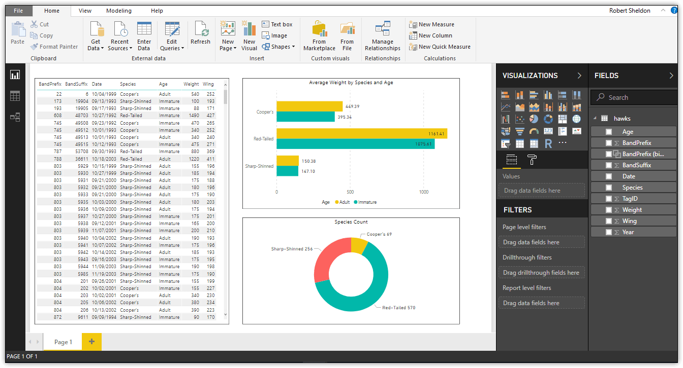
To access any of the three views, click the applicable button in the left navigation pane. The following figure shows Power BI Desktop with Report view selected, displaying a one-page report with three visualizations.

When working in Power BI Desktop, you will normally perform the following four basic steps, although not necessarily in a single session:

1. Connect to one or more data sources and retrieve the necessary data.

2. Transform and enhance the data using Data view, Relationships view, or the Query Editor, as necessary.

3. Create reports based on the transformed data, using Report view.

4. Publish the reports to the Power BI service or upload them to Power BI Report Server.

This article will focus primarily on steps 1 and 2 so you can get a better sense of how to retrieve and prepare the data, which is essential to building comprehensive reports. Later in the series, you’ll learn more about building reports with different types of visualizations, but first you need to make sure you get the data right.

Connecting to Data in Power BI Desktop

Power BI Desktop supports connectivity to a wide range of data sources, which are divided into the following categories:

• All: Every data source type available through Power BI.

• File: Source files such as Excel, CSV, XML, or JSON.

• Database: Database systems such as SQL Server, Oracle Database, IBM DB2, MySQL, SAP HANA, and Amazon Redshift.

• Azure: Azure services such as SQL Database, SQL Data Warehouse, Blob Storage, and Data Lake Store.

• Online Services: Non-Azure services such as Google Analytics, Salesforce Reports, Facebook, Microsoft Exchange Online, and the Power BI service.

• Other: Miscellaneous data source types such as Microsoft Exchange, Active Directory, Hadoop File System, ODBC, OLE DB, and OData Feed.

To retrieve data from one of these data sources, click the Get Data button on the Home ribbon in the main Power BI window. This launches the Get Data dialog box, shown in the following figure.

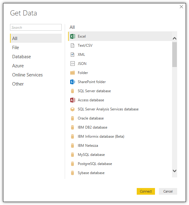
To access a data source, navigate to the applicable category, select the source type, and click Connect. You will then be prompted to provide additional information, depending on the data source. This might include connectivity details, an instance or file name, or other types of information. After you provide the necessary details, Power BI Desktop will launch a preview window that will display a sample of the data along with additional options.

This article uses a CSV file based on data from the Hawks dataset, which is available through a GitHub collection of sample datasets. The Hawks dataset contains data collected over several years from a hawk blind at Lake MacBride near Iowa City, Iowa. Name the file hawks.csv and save it to a local folder (C:\DataFiles).

To import the data from the file into Power BI Desktop, select the Text/CSV data source type in the Get Data dialog box. Click Connect and the Open dialog box will appear. From there, navigate to the C:\DataFiles folder, select the hawks.csv file, and click Open. This launches the preview window shown in the following figure.

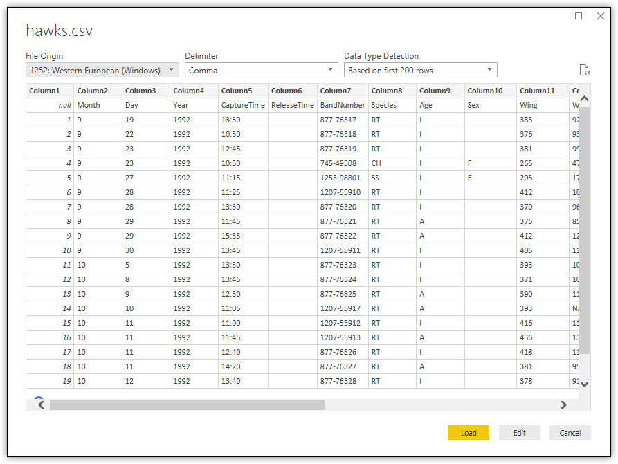
In addition to being able to preview a subset of the data, you can configure several options: File Origin (the document’s encoding), Delimiter, and Data Type Detection. In most cases, you’ll be concerned primarily with the Data Type Detection option. By default, this is set to Based on first 200 rows, which means that Power BI Desktop will convert the data to Power BI data types based only on the first 200 rows of data.

This might be okay in some cases, but there could be times when a column includes a value different from the majority of values, but that value is not in the first 200 rows. As a result, you could end up with a suboptimal data type or even an error. To avoid this risk, you can use the Data Type Detection option to instruct Power BI Desktop to base the data type selection on the entire dataset, or you can instead forego any conversion and keep all the data as string values.

You can also edit the dataset before loading it into Power BI Desktop. When you click the Edit button, Power BI Desktop launches Query Editor, which provides a number of tools for transforming data. After you make the changes, you can then save the updated dataset.

In this case, load the data into Power BI Desktop without changing any settings or editing the dataset. You will be transforming the data later as part of working through this article. To import the data as is, you need only click the Load button. You can then view the imported dataset in Data view, as shown in the following figure.

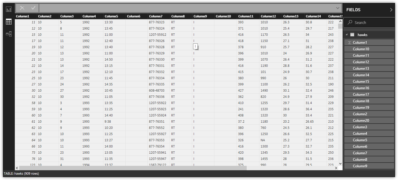
After you import a dataset into Power BI Desktop, you can use the data in your reports as is, or you can edit the data, applying various transformations and in other ways shaping the data. Although you can make some modifications in Data view, such as being able to add or remove columns or sort data, for the majority of transformations, you will need to use Query Editor, which includes a wide range of features for shaping data.

Introducing Query Editor

To launch Query Editor, click the Edit Queries button on the Home ribbon. Query Editor opens as a separate window from the main Power BI Desktop window and displays the contents of the dataset selected in the left pane, as shown in the following figure. In this case, the pane includes only the hawks dataset, which is the one you just imported.

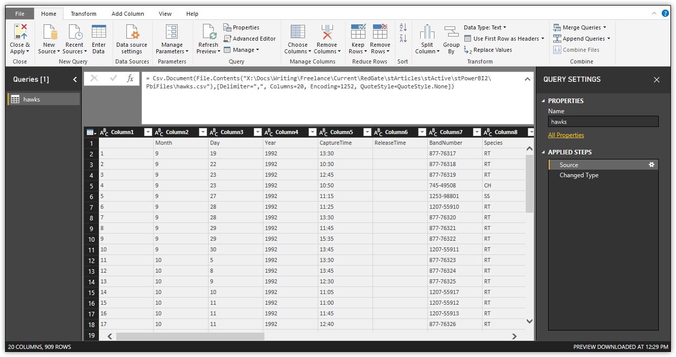
The dataset itself is displayed in the main pane of the Query Editor window. You can scroll up and down or right and left to see all the data. The pane to the right, which is separated into two sections, provides additional information about the dataset. The Properties section displays the dataset’s properties. In this case, the section includes only the Name property. To view all properties associated with a dataset, click the All Properties link within that section.

The Applied Steps section lists the transformations that have been applied to the dataset in the order they were applied. Each step in this section is associated with a script statement written in the Power Query M formula language. The statement is shown in the formula bar directly above the dataset. (If the formula bar is not displayed, select the Formula Bar checkbox on the View ribbon to display it.)

Currently, the Applied Steps section for the hawks dataset includes only two steps: Source and Changed Type. Both steps are generated by default when importing a CSV file. The Source step corresponds to the following M statement (provided here in case you cannot read it in the above figure):

The M statement consists primarily of the connection string necessary to import the hawks.csv file. Notice that it includes the delimiter and encoding specified in the preview window, along with other details.

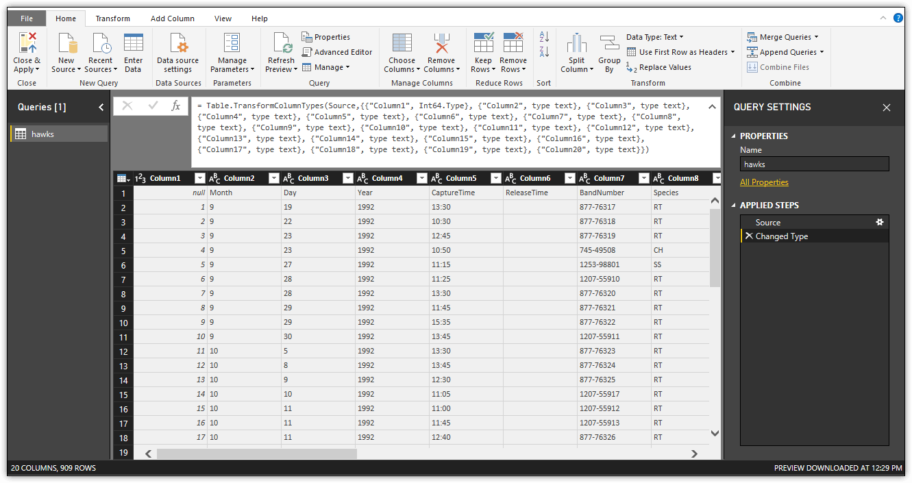
The second step, Changed Type, converts the data in each column to Power BI data types. The step is associated with the following M statement, which shows that the first column is assigned the Int64 type and that all other columns are assigned the text type:

If you had opted to forego data type conversions when importing the hawks.csv file, all columns would be assigned the text data type, but you instead stuck with the Based on first 200 rows option, which resulted in one column being converted to the Int64 type. The following figure shows the dataset with the Changed Type step selected and its associated M statement in the formula bar.

This article won’t spend much time on the M language. Just know that the language is the driving force behind the Power BI Desktop transformations in Query Editor. Articles later in this series will dig into the language in more detail so you can work with it directly.

Every transformation you apply to a dataset is listed in the Applied Steps section, and each step is associated with an M statement that builds on the preceding step. You can use the steps and their associated M statements to work with the dataset in various ways. For example, if you select a step in the Applied Steps section, Query Editor will display the dataset as it existed when the step was applied. You can also modify steps, delete steps, inject steps in between others, or move steps up or down. In fact, the Applied Steps section is one of the most powerful tools you have for working with Power BI Desktop datasets. Be aware, however, that it’s very easy to introduce an error into the steps that turns all your work into a big mess.

With that in mind, you’ll next provide column names for the dataset. You might have noticed from the screenshots—or when you imported the data for yourself—that the first row of data contains the original column names. This is why all columns but the first were assigned the text data type, even if most values were numbers. The first column was assigned the Int64 data type because it was the index for the original dataset and did not require a column name.

To convert the first row into columns names, click the Use First Row as Headers button on the Home ribbon. Power BI Desktop will promote the row and add a Promoted Headers step to the Applied Steps section, as well as a Changed Type step, which converts the data types of any fields that might be impacted by removing the column names as data values.

The following M statement is associated with the Changed Type step added to the hawks dataset:

Notice that, in addition to the first column, several other columns have been converted to the Int64 data type. However, the Wing column has been converted to the number type because it contains at least one decimal value. Other columns retained the text data type because they contained only character values or contained a mix of types.

It should be noted that the Changed Type step just added to the hawks data set is actually named Changed Type1. If a step is added that is of the same type as a previous step, Query Editor tags a numerical value to onto the new step to differentiate its name from the earlier step.

To complete the process of promoting the first row to headers, you might need to rename one or more columns. For example, because the hawks dataset did not include a name for the first column, change it from the auto-generated column1 name to TagID, as shown in the following figure by right-clicking into the column1 heading and selecting Rename.

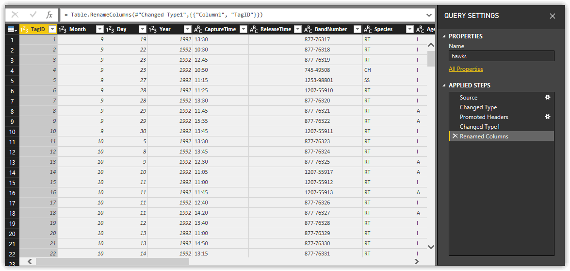
As you can see, the Applied Steps section now includes the Renamed Columns step. Also notice that each column name is preceded by a symbol that indicates the column’s data type. If you click the symbol, a context menu will appear and display a list of symbols and their meanings. You can also change the data type from this menu.

Note, however, that the name of the data types listed here are not always the same as the names used in the M statements. For example, the Int64 data type that appears in the M statements is listed as the Whole Number data type in the context menu.

Addressing Errors

When working in Query Editor, you might run into errors when converting data, modifying applied steps, or taking other actions. Often you won’t realize that there is an error until you try to apply any changes you’ve made. (You should be applying and saving your changes regularly when transforming data.)

To apply your changes in Query Editor, click the Close & Apply down arrow on the Home ribbon, and then click Apply. Any changes that you made since they last time you applied changes will be incorporated into the dataset, unless there is an error. For example, when you apply the changes to the hawks dataset after promoting the headers, you will receive the message shown in the following figure.

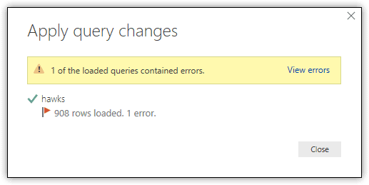
When you click the View errors link, Query Editor will isolate the row that contains the error, as shown in the following figure. The TagID value for this row is 263. After viewing the error row, you should see that the Wing column contains an NA value, although the column is configured with the number data type, which is why you received the error.

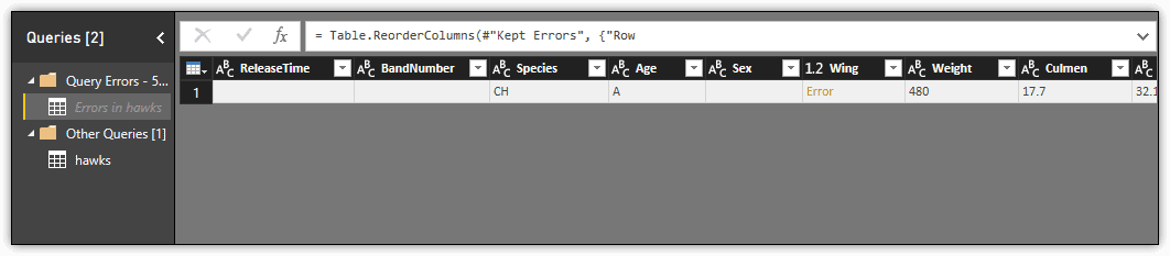
Click hawks on the left to exit out of the Errors screen and get back to the Query Editor.

To address an error in Query Editor, you can replace or remove the error or change the column’s data type:

• To change the column’s type, click the type icon next to the column name, and then click Text.

• To replace the error, right-click the column header, click Replace Errors, type a replacement value, and then click OK.

• To filter out the row with the error, click the down arrow next to the TagID header, search for the 263, and then clear the checkbox associated with this ID.

• To remove all rows that contain errors, click the table icon in the top left corner of the data set, and then click Remove Errors. This is the approach I took for the hawks dataset. As a result, the Removed Errors step was added to the Applied Steps section.

Removing Columns

In some cases, the data you import includes columns that you don’t need for your reports. Query Editor makes removing these columns a simple and quick process:

• To remove a single column, select the column directly in the displayed dataset, and then click the Remove Columns button on the Home ribbon, or you can instead right-click the column header and then click Remove.

• To remove multiple columns, select the first column, press and hold the Control key, select each additional column, and then click the Remove Columns button on the Home ribbon.

For the hawks dataset, remove the following columns because they are not relevant to the reports you might create or they contained numerous NA values:

• CaptureTime

• ReleaseTime

• Sex

• Culmen

• Hallux

• Tail

• StandardTail

• Tarsus

• WingPitFat

• KeelFat

• Crop

After removing the columns, Query Editor adds a single Removed Columns step to the Applied Steps section, as shown in the following figure.

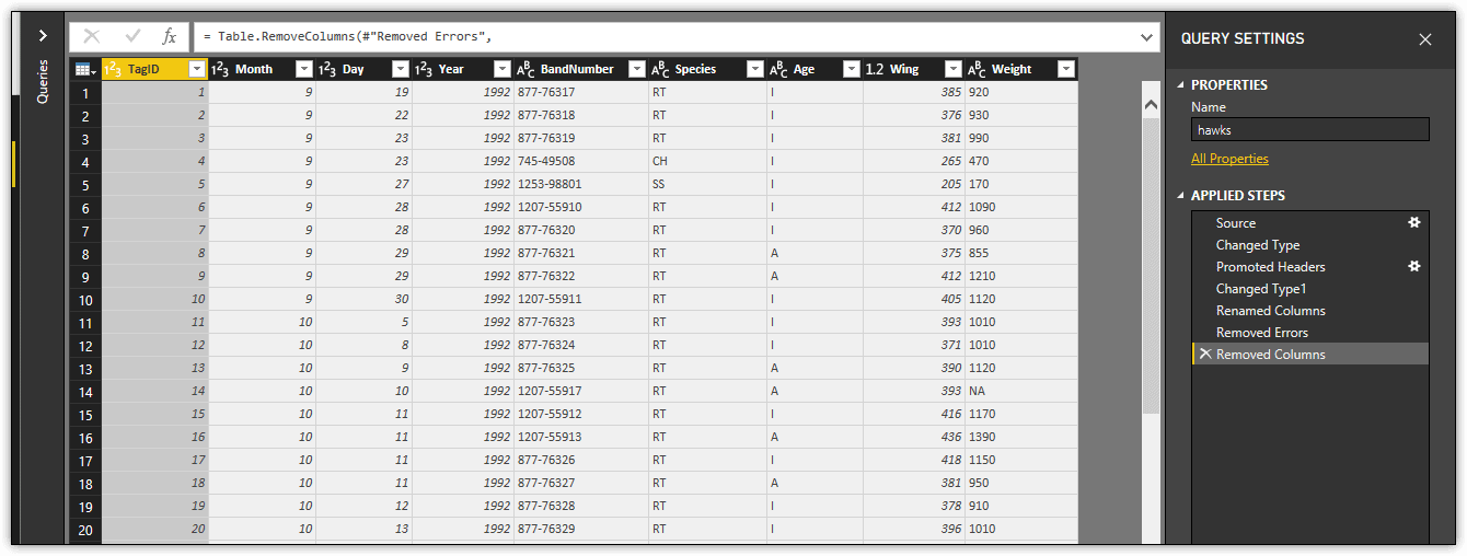
One of the advantages of having the Removed Columns step listed along with the other steps is that you can easily remove or modify the step if you later decide that one or more of the columns should not have been removed. In this case, you’re relatively safe modifying this step because any steps that you might have added after deleting the columns cannot reference those columns because they’re considered nonexistent. Close the Query Editor to go back to Data view.

Adding a Calculated Column

With Power BI Desktop, you can add calculated columns to a dataset that concatenates data or performs calculations. Power BI Desktop provides two methods for adding a calculated column. The first is to create the column in Data view, using the Data Analysis Expressions (DAX) language to define the column’s logic.

To create a DAX-based column, click the New Column button on the Home ribbon in Data view, and then type the DAX expression in the formula bar at the top of the dataset. The new column should be selected when adding the expression. After you type the expression, click the checkmark to the left of the expression to verify the syntax and populate the new column.

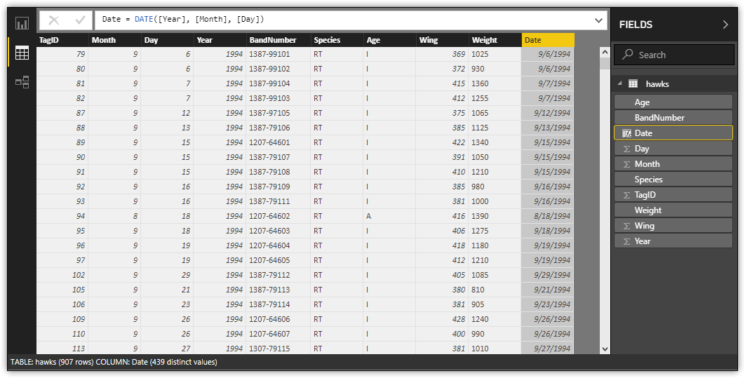
For example, add a column named Date to the hawks dataset to provide a single value that shows the date when a hawk was tagged, using the following DAX expression:

The expression uses the DATE function to create a date value based on the Year, Month, and Day columns. After you add the Date column, you can set the displayed format. Go to the Modeling ribbon in Data view, click the Format drop-down list, point to Date Time, and click 3/14/2001 M/d/yyyy. The following figure shows the new column after I added it to the dataset, with the applied format.

Using DAX to create a column in Data view is quick and easy. However, this approach has some limitations. For example, the column is not available in Query Editor, so it cannot be used as part of another calculated column definition in Query Editor. In addition, if you delete a column referenced by a DAX expression, the values in the DAX-based column will show only errors.

The safest way to get around these limitations is to create your column in Query Editor. Delete the Date column you just added in the Data view. Click Edit Queries to reopen the Query Editor. Click the Custom Column button on the Add Column tab. When the Custom Column dialog box appears, type a name for the new column and the column’s formula, which is an M expression that defines the column’s logic. (Query Editor automatically adds the rest of the M syntax to create a complete statement.) For example, to create a column like the DAX-based column above, used the following M expression:

The statement uses the #date method to create a date value based on the Year, Month, and Day columns, similar to the DAX expression. The following figure shows what the M expression looks like when entered into the Custom Column dialog box.

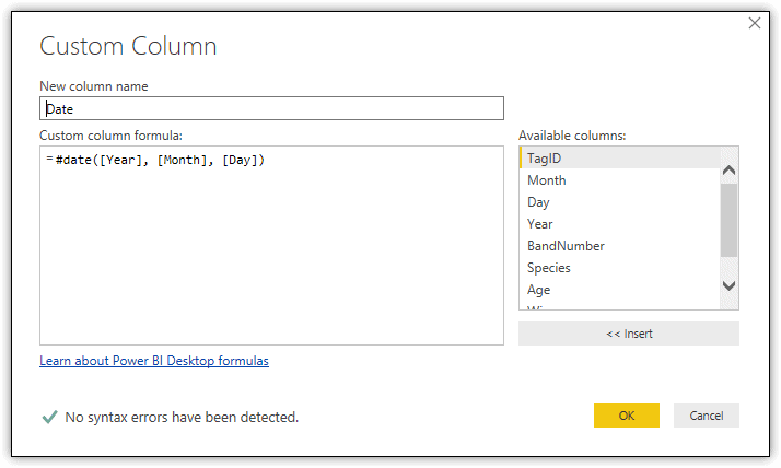
When entering your M expression in the Custom Column dialog box, be sure that the green arrow is showing at the bottom of the dialog box to ensure that there are no syntax errors. Be aware, however, that you can have errors in your M statement without them showing up as syntax errors.

When you create a calculated column, Query Editor adds the Added Custom step to the Applied Steps section. You can then reference the new column in other calculated columns. You can also remove any of the columns referenced by the M expression. In this case, remove the Month and Day columns but keep the Year column in case you want it available for reports.

Splitting a Column

In Query Editor, you can split a column based on a specified value (delimiter) or by a specified number of characters. For example, the hawks dataset includes the BandNumber column, which is made up of two parts, separated by a hyphen. One of those parts might have special meaning, such as indicating the individual who tagged the hawk or the process used to tag the hawk. Splitting the column could make it easier to group the data by a particular entity.

To split a column by a delimiter, right-click the column’s header, point to Split Column, and then click By Delimiter. In the Split Column by Delimiter dialog box, specify the delimiter and then click OK. Query Editor will split the column into two columns (removing the delimiter) and update the data types if necessary. You can then rename the columns if you do not want to use the autogenerated names.

The following figure shows the hawks dataset after splitting the BandNumber column and changing the names of the two new columns to BandPrefix and BandSuffix.

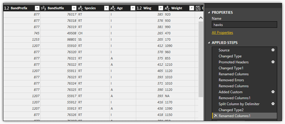
Notice that three steps have been added to the Applied Steps section: Split Column by Delimiter, Changed Type2, and Renamed Columns1.

Performing Additional Data Transformations

When you’re preparing a dataset for reporting, you should evaluate the data types that have been assigned to each column to ensure they’re what you need. Usually you’ll want to hold off doing this until after you’ve added, removed, or split columns so you’re not introducing unnecessary transformation steps. Evaluating the data types can also point to possible anomalies in the data.

For example, the BandPrefix column was assigned the number data type, which would have been expected to be the Int64 data type. The same goes for the Wing column. In addition, the Weight column was assigned the text data type, and the Date column was assigned the Any data type. For this article, change the data types for the BandPrefix, Wing, and Weight columns to the Int64 data type (whole number), and change the Date column to the date data type.

The reason the Wing column was assigned the number data type was because it contained a decimal value. When changing the data type to Int64, Query Editor automatically rounded the value to the nearest whole number, which worked fine for the purposes of this article.

The process was not quite as simple for the Weight column. The reason it was assigned the text data type was because the column contained NA values, which were treated as errors when changing the column to the Int64 data type. Remove these rows by using the Remove Errors option.

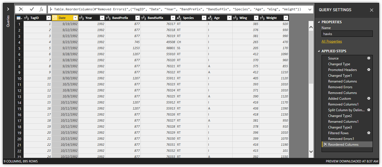
The next step is to move the Date column left within the dataset so it appears before the Year column. To move a column in Query Editor, simply drag the column header to the new position. Query Editor will add the Reordered Columns step to the Applied Steps section, as shown in the following figure. The figure also shows the other steps that were added when changing data types, filtered rows, and removed errors.

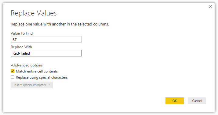
The final step is to replace the values in the Species and Age columns to make them more readable. To replace a value, right-click the column header, and click Replace Values. In the Replace Values dialog box, type the original value and new value in the applicable text boxes. Next, click the Advanced options arrow, and select the Match entire cell contents checkbox. This is important to ensure that you don’t replace part of another value.

The first value to replace in the hawks data set is the RT value in the Species column. For the new value, used Red-Tailed, as shown in the following figure.

Also replace the following values:

• The CH value in the Species column with Cooper’s.

• The SS value in the Species column with Sharp-Shinned.

• The A value in the Age column with Adult.

• The I value in the Age column with Immature.

The following figure shows the updated values in the Species and Age columns, as the dataset appears in the Data view of the main Power BI Desktop window.

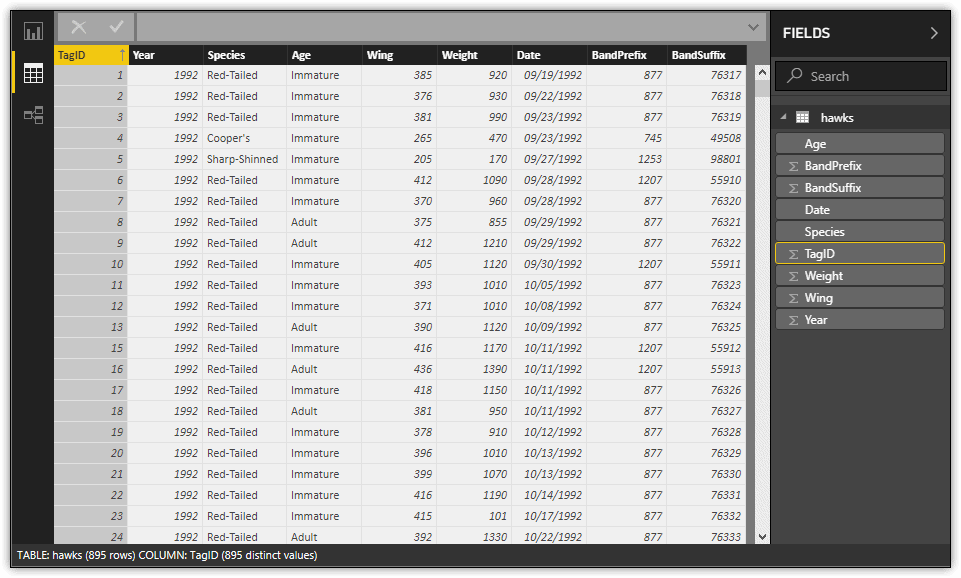
Notice that the columns are not impacted by the reordering that was done in Query Editor. The newer columns—Date, BandPrefix, and BandSuffix—are included at the right side of the dataset, after the original columns. Also notice that in this case the Date column is configured in the format mm/dd/yyyy, but you might see the data values spelled out or displayed in another format. However, you can choose any format from the Format drop-down list on the Modeling ribbon.

Generating Reports

Once you get your datasets in the format you want them, you can begin to create reports and their visualizations. Just to show you a sample of what can be done, I created one report with three visualizations based on the hawks data set, as shown in the following figure.

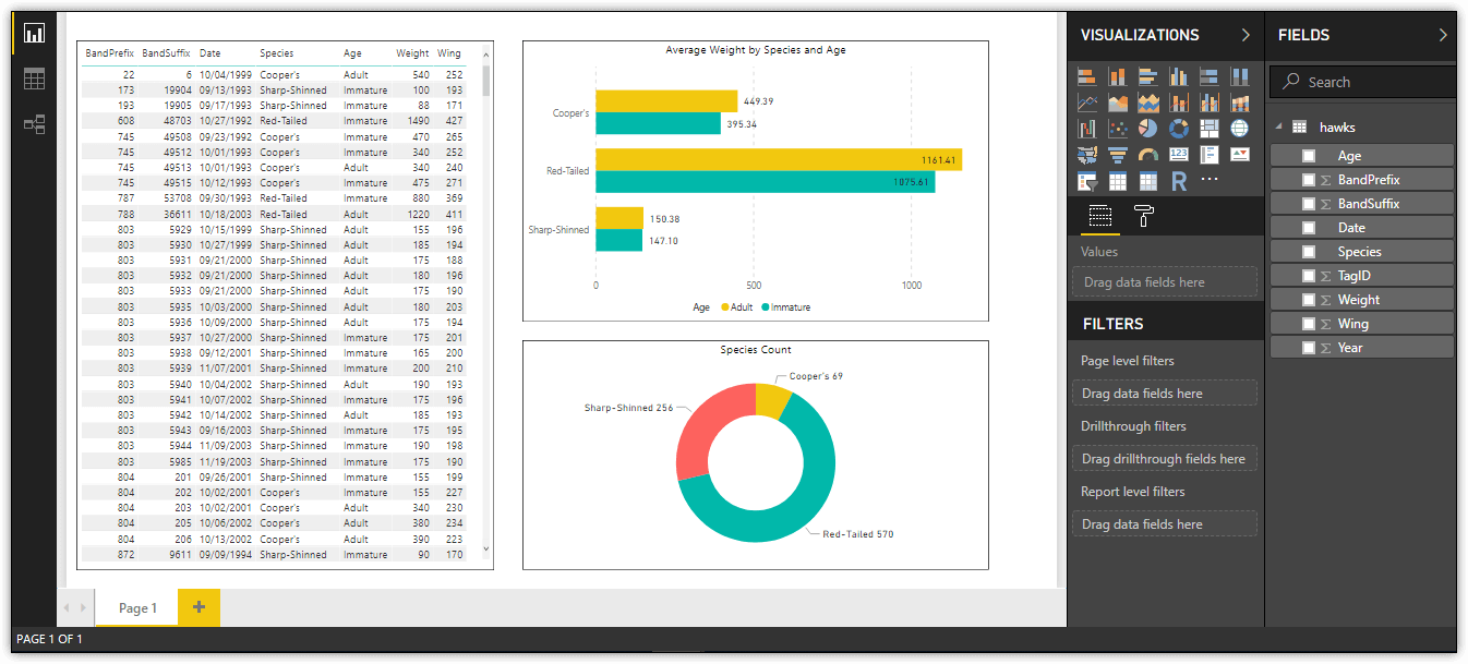
The figure contains a one-page report as it appears in Report view in Power BI Desktop. The report includes a table, bar chart, and donut chart, all based on the hawks dataset. Although this article doesn’t focus on reports, be aware that Report view includes a variety of options for creating and configuring different types of visualizations. Later in the series, you’ll learn how to create reports and visualizations and publish them to the Power BI service.

Working with Power BI Desktop

There’s much more you can do with Power BI Desktop and Query Editor than what was covered here. In addition to creating various types of visualizations, you can merge and append queries, group and aggregate data, pivot columns, define relationships, run R scripts, and carry out a number of other tasks. The best way to become familiar with these features is to experiment with them against different types of data. The better you understand how to work with Power BI Desktop, the more effectively you can use the rest of the Power BI tools, including the Power BI service, Power BI Report Server and the Power BI mobile apps.