

Lazy Spool
Just in case if you haven’t been following my articles, I’m writing a series about the SQL Server Showplan operators, and the next one on my list is the Lazy Spool operator. If you missed the last article talking about Eager Spool, it’s actually very important that you read that before you get too deeply into this next article. If you’re just getting started with my Showplan series, you can find a list of all my articles here.
I know it’s been two weeks since my last “weekly article” but, as much as I generally don’t like excuses, the last few weeks really were very busy for me. With the help of a lot of coffee nd fast food (IT Professionals have to eat at least once in a blue moon), I’ve been teaching 4-hour SQL Server classes every evening, snatching a few hours of sleep where I can, and having bizarre dreams about Clustered Indexes shooting flying Showplan Operators with automatic weapons. I love my life, but sometimes, just sometimes, I take on too much.
The Lazy Spool is actually very similar to the Eager Spool; the difference is just that Lazy Spool reads data only when individual rows are required. It create a temporary table and build this table in a “lazy” manner; that is, it reads and stores the rows in a temporary table only when the parent operator actually asks for a row, unlike Eager Spool, which reads all rows at once. To refer back to some material I covered in the Eager Spool explanation, the Lazy Spool is a Non-blocking operator, whereas Eager Spool is a Blocking Operator.
To highlight the Lazy Spool, we’ll create a table called Pedidos (which means “Orders” in Portuguese). The following script will create a table and populate it with some garbage data:
|
1 2 3 4 5 6 7 8 9 10 11 12 13 14 15 16 17 18 19 20 21 22 23 24 25 26 27 28 29 30 31 32 33 34 35 36 37 38 39 40 41 42 |
IF OBJECT_ID('Pedido') IS NOT NULL DROP TABLE Pedido GO CREATE TABLE Pedido (ID INT IDENTITY(1,1) PRIMARY KEY, Cliente INT NOT NULL, Vendedor VARCHAR(30) NOT NULL, Quantidade SmallInt NOT NULL, Valor Numeric(18,2) NOT NULL, Data DATETIME NOT NULL) DECLARE @I SmallInt SET @I = 0 WHILE @I < 50 BEGIN INSERT INTO Pedido(Cliente, Vendedor, Quantidade, Valor, Data) SELECT ABS(CheckSUM(NEWID()) / 100000000), 'Fabiano', ABS(CheckSUM(NEWID()) / 10000000), ABS(CONVERT(Numeric(18,2), (CheckSUM(NEWID()) / 1000000.5))), GETDATE() - (CheckSUM(NEWID()) / 1000000) INSERT INTO Pedido(Cliente, Vendedor, Quantidade, Valor, Data) SELECT ABS(CheckSUM(NEWID()) / 100000000), 'Amorim', ABS(CheckSUM(NEWID()) / 10000000), ABS(CONVERT(Numeric(18,2), (CheckSUM(NEWID()) / 1000000.5))), GETDATE() - (CheckSUM(NEWID()) / 1000000) INSERT INTO Pedido(Cliente, Vendedor, Quantidade, Valor, Data) SELECT ABS(CheckSUM(NEWID()) / 100000000), 'Coragem', ABS(CheckSUM(NEWID()) / 10000000), ABS(CONVERT(Numeric(18,2), (CheckSUM(NEWID()) / 1000000.5))), GETDATE() - (CheckSUM(NEWID()) / 1000000) SET @I = @I + 1 END SET @I = 1 WHILE @I < 3 BEGIN INSERT INTO Pedido(Cliente, Vendedor, Quantidade, Valor, Data) SELECT Cliente, Vendedor, Quantidade, Valor, Data FROM Pedido SET @I = @I + 1 END GO |
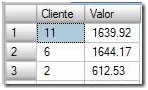
This is what the data looks like:
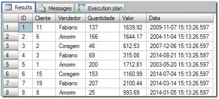
Figure 1. The demonstration data we’ll be working with in this article.
To understand the Lazy Spool, I wrote a query that returns all Orders where the Order value is lower than the average value of all the relevant customer’s orders. That sounds a little convoluted, so let’s just look at the query:
|
1 2 3 4 5 6 |
SELECT Ped1.Cliente, Ped1.Valor FROM Pedido Ped1 WHERE Ped1.Valor < ( SELECT AVG(Ped2.Valor) FROM Pedido Ped2 WHERE Ped2.Cliente = Ped1.Cliente) |
Before we see the execution plan, let’s make sure we understand the query a little better. First, for each customer in the FROM table (Ped1.Cliente), the SubQuery returns the average value of all orders (AVG(Ped2.Valor)). After that, the average is compared with the principal query and used to filter just each customer’s orders with values lower than their average.
So, now we’ve got the following execution plan:
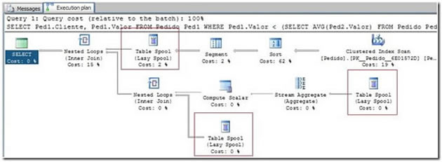
Figure 2. The execution plan generated by the example query.
And here’s the text version of the Execution Plan:
|
1 2 3 4 5 6 7 8 9 10 11 12 |
|--Nested Loops(Inner Join) |--Table Spool | |--Segment | |--Sort(ORDER BY:([Ped1].[Cliente] ASC)) | |--Clustered Index Scan(OBJECT:([Pedido].[PK__Pedido__6E01572D] AS [Ped1])) |--Nested Loops(Inner Join, WHERE:([Pedido].[Valor] as [Ped1].[Valor]<[Expr1004])) |--Compute Scalar(DEFINE:([Expr1004]=CASE WHEN [Expr1012]=(0) THEN NULL ELSE | [Expr1013]/CONVERT_IMPLICIT(numeric(19,0),[Expr1012],0) END)) | |--Stream Aggregate(DEFINE:([Expr1012]=Count(*), | [Expr1013]=SUM([Pedido].[Valor] as [Ped1].[Valor]))) | |--Table Spool |--Table Spool |
As we can see, the Spool operator is displayed three times in the execution plan, but that don’t mean that three temporary tables were created. All the Spools are actually using the same temporary table, which can be verified if you look at the operator’s hints displayed in the graphical execution plan:
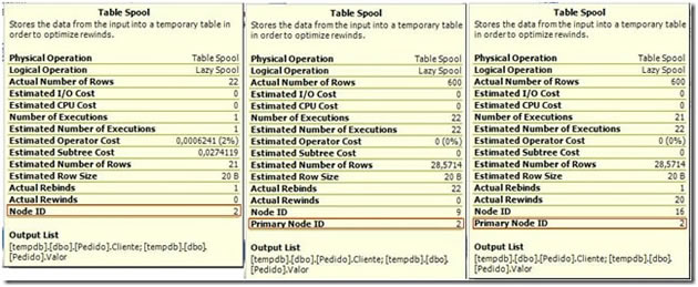
Figure 3. Comparison of the three instances of Lazy Spool in our execution plan.
As you can see, the first Spool hint has the Node ID equal to 2, and the other two operators are referenced to the Primary Node 2 as well. Now let’s look at a step by step describe the execution plan so that we can understand exactly what it is doing. Note this is not the exact order of execution of the operators, but I think you’ll understand things better in this way.
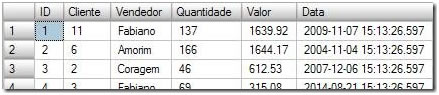
The first step in the execution plan is to read all of the data that will be used in the query, and then group that data by customer:
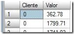
 The Clustered Index Scan operator reads all rows from the Cliente and Valor (Client and Value) columns. So, the Input of this operator is the following:
… and the Output is just the Client and Value columns:
 When the Sort operator receives the rows from the clustered index scan, it’s output is all the data, ordered by the Client column:
 The Segment operator divides the data into many groups; in this case it receives all the rows, ordered by customers, and divides them into groups that share the same costumer. So, the first segment produced by this operator will be all the rows where “Client = 0“. Given that the data is already sorted by customers, the operator just needs to read down the rows until it finds a different value in order to create a segment. When the value it is reading changes, it finishes its job and the next operator immediately receives the segment of all the data for “Customer 0”. This process will repeat until all segments are completely read. The final output of the Segment operator is a series of segments dividing all the data according to customer, such that each segment contains all the rows for a particular customer. In this walkthrough, we’ll look at all the rows where “Client=0“:

 Here we get on to the Table Spool operator, working as a “Lazy” Spool. It will create a temporary table in the TempDB database, and store all data returned from the Segment operator; in this case, all the data for customer 0. The output of the Spool operator is just all data stored in the tempdb table.
  The Nested Loops operator joins the first and second parts of the execution plan, or rather, the principle query with the subquery. As we now, the nested loops scan a table and join it with another table one row at time, and so for each row in the Table Spool (Item 4) the nested loop will join the result of Item 11. To give you a quick preview, this result will be the rows where the Value column in the Spool table is lower than the value calculated in the aggregation (Item 8 – the average value of the customer’s orders). When this step is finished, the Spool operator (item 4) is called again, and it in turn calls the Segment operator, which reads another segment of rows (i.e. processes another customer). This cycle repeats until all rows are read.
Now, let’s to go to the second part of this plan, which will run the SubQuery that returns the average order value for one costumer.
- To start with, the execution plan reads the data from the Lazy Spool and passes the results to the aggregate to calculate the average. Remember that the rows in the Spool operator are currently only the rows for “Customer 0”.
 The Stream Aggregate operator will calculate the average of the value column, returning one row as an Output value.
 The Compute Scalar operator will convert the result of the aggregation into a Numeric DataType, and pass the Output row to the Nested Loops operator in Step 9.
- The last table spool is used to once again read the “Client=0” rows from the Spool table, which will be joined with the result of the compute scalar.
- The Nested Loops operator performs an iterative inner join; in this case, for each row returned by the computed scalar, it scans the Spool table and returns all rows that satisfy the condition of the join. Specifically, it returns the rows where the Value column in the Spool table is lower than the value calculated in the aggregation.
Quick Tip:
If you create an index on the Pedidos table covering the Client column and include the Value column, you will optimize the query because the Sort operator will not be necessary, and it costs 62% of the whole query.
We saw that the Query Optimizer can use the Lazy Spool operator to optimize some queries by avoiding having to read the same values multiple times. Because SQL Server uses the Spool Lazy, the SQL works with just one chunk of the data in all operations, as opposed to having to constantly fetch new data with each iteration. Clearly, that translates into a great performance gain. Keep your eyes open to see more about the Spool operators, as we still need to feature the NonClustered Index Spool and the RowCount Spool!
That’s all folks; I’ll see you next week with more “Showplan Operators”.
If you missed the last thrilling Showplan Operator, Eager Spool, you can see it here.