The series so far:

1. How to query blob storage with SQL using Azure Synapse
2. How to query private blob storage with SQL and Azure Synapse
3. Performance of querying blob storage with SQL 

When you deal with Big Data in Azure, you will store lots of files on Azure Storage. From time to time, you may need to investigate these files. Wouldn’t it be cool if you could just open a window and execute a SQL Query over the storage? In this article, I explain how to query blob storage with SQL using Azure Synapse.

Synapse Analytics makes this not only possible but also very affordable since you pay as you go. At the time of this writing, it estimates only $5.00 USD for each terabyte processed. Synapse Analytics makes it easy to query your storage and analyse files using the SQL language.

Disclaimer: This is only the price for data processing on the Synapse Serverless SQL pool. It doesn’t include the storage price and other services used. This price may change anytime. Please, check the pricing on the Azure website for more precise information.

Next, I’ll show you how to implement Azure Synapse and dig into the details to show you how it works.

Provisioning the workspace

I will not duplicate the good Microsoft documentation. You can follow this QuickStart to provision the workspace. Use the option to create a new storage account together with the workspace.

When the workspace is provisioned, only the SQL On Demand pool is created. It’s the most affordable one, and you can stick to that: use the SQL On Demand pool to query your blob storage.

The Synapse Workspace name needs to be unique because It can become a public URL. In fact, it is one by default. I will call my Synapse Workspace MaltaLake. You need to create your own custom name for your Synapse Workspace. Every time I refer to MaltaLake, replace it with your workspace name.

Provisioning a storage account

The storage account you created in the previous step will be used by Synapse Analytics itself for things like metadata. In order to make a demonstration of a small data lake, you will need another storage account.

During the example, I will call the storage LakeDemo. This is the name for my storage, which also needs to be unique. You will need to create a unique name for your storage and use it every time you run an example that uses LakeDemo by adjusting the scripts, replacing LakeDemo with your storage account name.

You can use a PowerShell script to provision the storage account and upload demo files to it. You can download the scripts and demos and execute the file Install.bat. It will ask you some questions and create the environment on your Azure account.

This is what the script will do for you:

• Create a resource group or use the existing resource group you provide
• Create a storage account or use an existing storage account you provide
• Upload the files to the storage account

If you would like, you can also follow these steps to provision a new storage account. You can still run the script after this, providing the name of the resource group and the storage account. The script will create the containers and upload the file.

Once again, if you would like, you can create the containers and upload the files by yourself. You will need two containers for the demonstrations, one private and one with public access: DataLake and OpenDataLake. In order to upload the files, you can use Azure Storage Explorer if you chose not to use the script.

Querying the blob storage data

Azure provides a nice environment, Synapse Studio, for running queries against your storage. Next, I’ll show you how to get started.

Opening the environment

Follow these steps to learn the details of Synapse Studio and how you will run these queries.

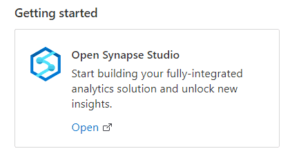
1. Open Azure Synapse Studio. You will find it under Getting Started on the Overview tab of the MaltaLake workspace

Synapse studio may ask you to authenticate again; you can use your Azure account.

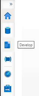
2. Open the Develop tab. It’s the 3^rd icon from the top on the left side of the Synapse Studio window

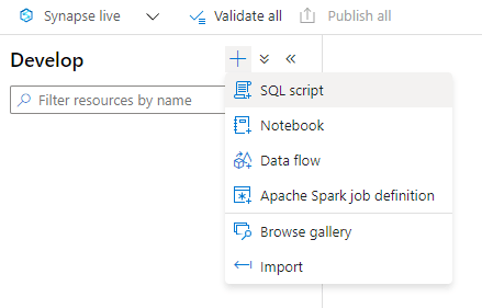
3. Create a new SQL Script
   1. On the Develop window, click the “+” sign
   2. Click the SQL Script item on the menu

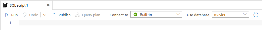
The script will be connected to BuiltIn, meaning the SQL On Demand. There are two databases, master and default. You can’t create objects in either of them.

A side note about scripts

You can save your scripts in Synapse. The button Publish on the image above is used to save your scripts. It is recommended that you change the name of your script before publishing because many scripts called SQL Script X can become confusing very fast.

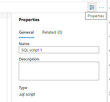
You can use the Properties window on the right side of the screen. It appears by default, but if hidden, the button on the toolbar, exactly over where the window should be, will make it appear again.

Synapse Studio also has additional features to manage the scripts. These features are hidden on the “…” menu each script type has. Once you click the “…”

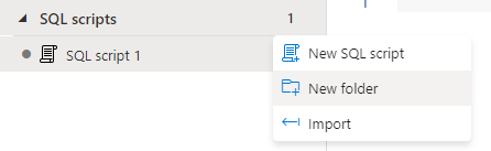
New Folder: You can organize scripts in folders under the script type. The Script type (“SQL scripts”) can have many folders under it.

Import: You can import existing scripts from your machine to Synapse Studio

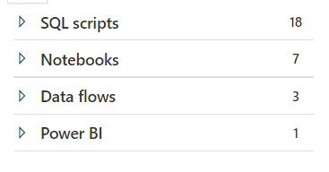
Besides these features, Synapse Studio also automatically breaks down the content according to the type of the script. For example, the image below is an example of a Develop environment with many kinds of elements.

File Type Support

Azure Synapse can read two types of files:

PARQUET: A columnar format with defined data types for the columns, very common in Big Data environments

CSV: The classic Comma Separated Values file format, without specified data types for the columns.

These file types can be in their regular format or compressed. The two possible compressions available are:

Snappy: Usually used with PARQUET

GZIP: Usually used with CSV

Work-Around for additional types

You can play around with CSV confirmation, defining the row and column delimiters to access different file types. The idea is simple: Read the entire files into a varchar(max) field and then use T-SQL features to process these fields.

For example, this works for JSON file types. After reading the files, you can process the fields using JSON functions.

Reading Parquet files

Copy the following query to the new script window created and execute the query. Don’t forget to change the URL to your storage URL:

The OPENROWSET function allows reading data from blob storage or other external locations. It works only with SQL On Demand pools; it’s not available with SQL Dedicated pools yet.

Usually, in data lakes, the data is broken down into many files, many pieces of data need to be loaded together as a single set. That’s why the URL is pointing to a folder. Synapse can read from all the files in the folder as if they are one. You don’t need to handle file-by-file; Synapse will return all the data. Beyond Synapse, this is a Big Data concept.

It’s also important that this URL finishes with “/”, otherwise it may be mistaken as a file. This requirement is not present for all statements that use an URL, but it’s better to always finish it with a “/”.

Another interesting rule is that Synapse will ignore any file inside the folder starting with “_” . This happens because many data lake tools use these files as metadata files to control the saving and ETL process, such as Azure Data Factory.

The OPENROWSET statement also defines the format as PARQUET. This is one of the formats very common on data lakes. Here are some characteristics of the PARQUET file:

• It includes not only column names but also types, but it has its own type system.
• It’s a columnar file, similar to ColumnStore indexes. This means it’s optimized to retrieve only the columns you ask for.
• It can be compressed using Snappy compression. OPENROWSET function automatically recognizes if it’s compressed or not.

Try one more query. You can create a new SQL script, or you can copy the query to the same script and select the query before executing it; it’s up to you.

Execute the following query:

This example is grouping, counting the taxi rides by month, and ordering. The use of functions over the date is not optimized at all, but still, this query executes in about one second. This query is an example showing more complex calculations and summaries from the data in the blob storage.

SQL Script execution features

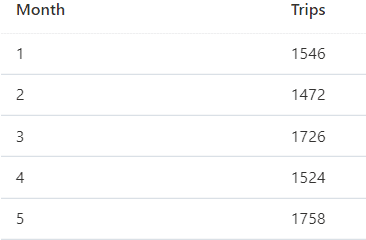
After executing the previous query, you can use some interesting features to better analyse the data. The query result, on the lower part of the window, is a list of months and the taxi trips made during that month.

Changing the view to Chart, you immediately see a line chart, as the image below:

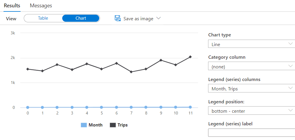
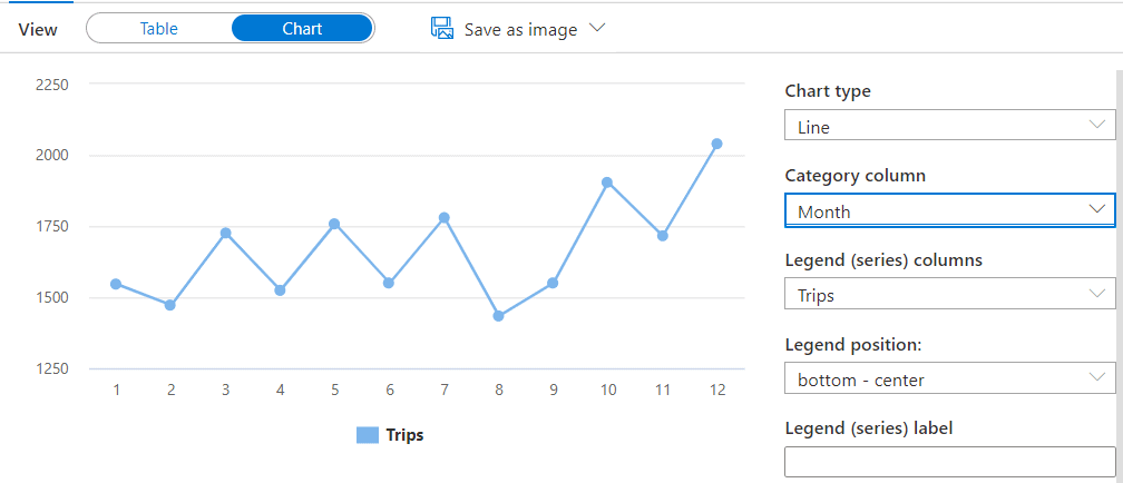
The chart is not correct. You may see Month and Trips fields are on the Legend space, which is not correct. The month should be a Category Column. Changing the Month to a Category column will make a big difference on the graphic, as you may note below.

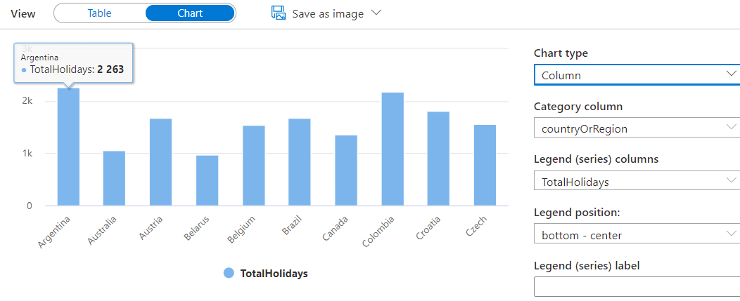
You can also change the type of chart to column, resulting in the image below:

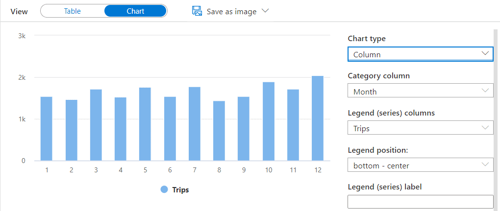
The possibility to query information on blob storage and other sources easily with a Serverless Pool has many uses. One of them is ad-hoc analysis queries, and the UI feature to view the result in many different ways contributes even more to this.

Reading CSV files

Copy the following query to a SQL script and execute it. Once again, you can create a new script, or you can use the same script and select the query before executing it.

This time, the query is trying to read CSV files. This example includes some additional information on the OPENROWSET function:

Field Terminator: The CSV format is flexible in relation to the characters used as field terminator, record terminator, and string delimiter. In this case, you are customizing only the field terminator.

First Row: This parameter tells to OPENROWSET function the records will start on the 2^nd line. When this happens, it’s usually due to the header of the columns, although not all CSV files have the column headers included.

Parser Version: There are more than one CSV parser available in Synapse. This example specifies the parser version 1.0.

After the execution, you will see an error message complaining it was not possible to identify the schema of the file.

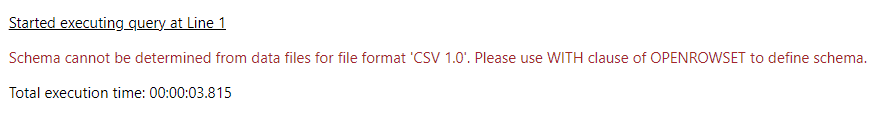
As opposed to the Parquet format, the CSV at most has the column names, never the types. This means that for the CSV files, you need to apply a technique called Schema-On-Read. You will apply the schema now, when reading the file, instead of applying it before, when the file was being saved.

You can specify the schema on the SELECT statement:

You may notice the WITH statement is considered part of the FROM clause, as if the entire OPENROWSET function and the WITH statement were only the table name. That’s why the table alias, AS [HOLIDAYS] only appears in the end.

Using Parser 2.0 for CSV files

Parser 2.0 has some interesting differences. Execute the same query as above, but now with parser 2.0:

You may notice the syntax has a small difference: instead of using the FirstRow parameter, it’s using the Header_Row parameter. In summary, the syntax is not the same between parser 1.0 and 2.0.

After the execution, some columns will return only NULL values. This is another difference with parser 2.0: It will make a match between the column names you use and the column names in the file. They need to match, otherwise, it’s like the columns you are specifying are new columns, not present in the file, so they are all filled with NULL.

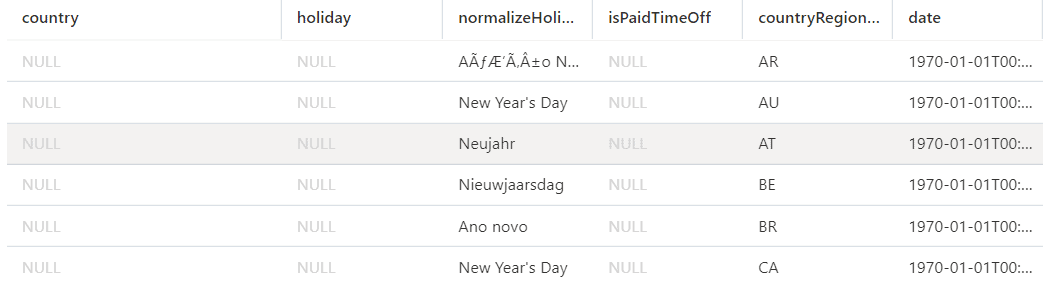
Luckily, parser 2.0 can also auto-detect the types in the CSV file. If you just remove the WITH clause, you will get back the existing fields in the file.

It’s interesting to notice this is basically the same query that failed under parser 1.0 because of the lack of field identification, while 2.0 auto-identifies the fields when possible. Not all CSVs have a header row, in this case, auto-identify the fields would be impossible.

In summary, this leaves three different ways to read CSV files:

• Using Parser 1.0 with schema
• Using Parser 2.0 with schema
• Using Parser 2.0 auto-detecting fields

Parser differences

Parser 1.0 Is created to be more feature complete, supporting more complex scenarios. Parser 2.0, on the other hand, is focused on performance and doesn’t have all the features Parser 1.0 has.

My recommendation is to use Parser 2.0 when it’s possible and revert to parser 1.0 when the feature is not available in 2.0.

A small summary about parser 2.0 extracted from https://docs.microsoft.com/en-us/azure/synapse-analytics/sql/develop-openrowset?WT.mc_id=DP-MVP-4014132:

“CSV parser version 2.0 specifics:

• Not all data types are supported.
• Maximum character column length is 8000.
• Maximum row size limit is 8 MB.
• Following options aren’t supported: DATA_COMPRESSION.
• Quoted empty string (“”) is interpreted as empty string.
• DATEFORMAT SET option is not honored.
• Supported format for DATE data type: YYYY-MM-DD
• Supported format for TIME data type: HH:MM:SS[.fractional seconds]
• Supported format for DATETIME2 data type: YYYY-MM-DD HH:MM:SS[.fractional seconds]”

Data types

The field identification makes the query much easier, but it’s important to be sure you are using the correct data types. CSV files don’t have data types for the fields, so the type identification may not be so precise; it doesn’t matter how much the Parser 2.0 has evolved in this area.

You can confirm by checking in detail the resultset returned using the sp_describe_first_result_set stored procedure. Execute this procedure passing a query as a parameter, like the example below:

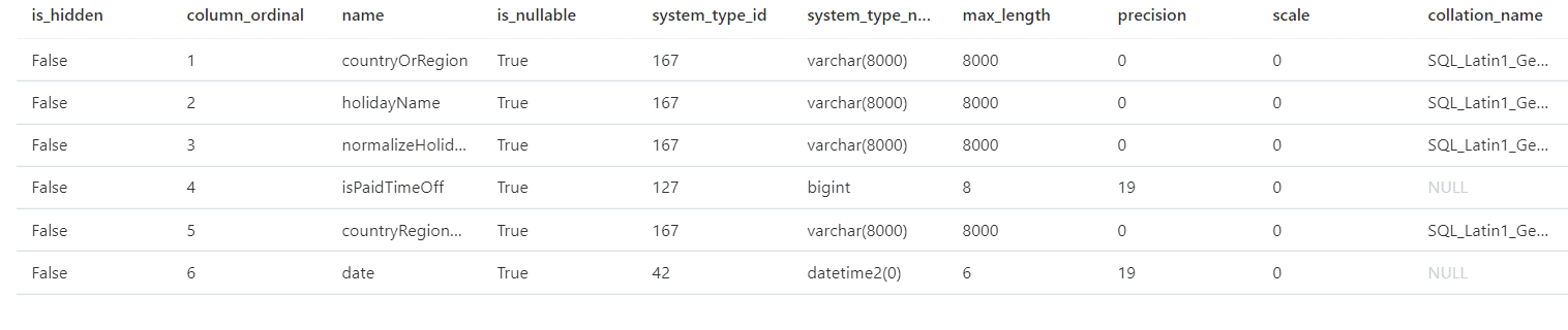
This stored procedure will help with many tasks in a data lake, discovering field names and data types. You may notice on the result of this execution, the field isPaidTimeOff was recognized as BigInt instead of Bit.

It’s important to be the most precise possible with the data types when using SQL over a data lake. Small mistakes will not prevent the query from working. The CSV format hasn’t types at all, while PARQUET format has a type system where some types can have more than one similar in SQL Server and there are no data type sizes.

Due to that, the query will work even with some mistakes, it’s just a matter of a data type conversion. However, you will pay the price of data type mistakes with slower queries. This is the worst kind of problem: The silent one, when everything seems to be working, but it’s charging you the performance cost.

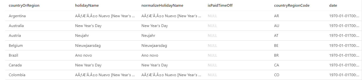
Even having the auto-detect feature, you can still override it to define better data types. You just need to keep the same column names, like on the query below:

This query above is not using the best data types possible yet. I will dig into the data types later.

Once again, you can make groupings and aggregations. Run this query to see how many holidays each country has:

Querying JSON files

JSON files are prevalent nowadays, and the need to query them is also very common in a data lake or data lake house.

A JSON file has elements and values separated by commas. It may appear strange, but this allows us to read a JSON file as a CSV file, resulting in a string, and later parsing the string as JSON. You use the CSV parser, then process the JSON using the OPENJSON function introduced in SQL Server 2017. In this way, you can retrieve specific data from the JSON files in your data lake.

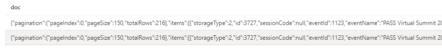
The query below makes the first step, read the JSON file. The classic JSON file uses the 0x0b terminator and the entire file is read as one row.

Each JSON file has a structure that, if broken, makes the JSON invalid. The query above will bring each file in the folder as a different record, keeping the JSON structure still valid.

After returning the records, you can use the OPENJSON function released in SQL Server 2017 to process the JSON. The query below does exactly this to extract some fields from the JSON.

Here are the highlights about the OPENJSON syntax:

• The first parameter is a JSON document in string format
• Use the cross apply, so you can execute the OPENJSON for each row retrieved from the previous query
• The 2^nd parameter of the OPENJSON function is a JSON expression applied from the root. The records will be the elements below this expression.
• You need to apply a schema to the data, but the field names are automatically matched with json properties. You will only need additional expressions if there isn’t a precise match, which doesn’t happen on this query.

How to query blob storage with SQL

In this first part of the series, you saw the basic concepts about using the Serverless Pool to query your blob storage. This is just the beginning. Next, I’ll go deeper about authentication, performance and conclude with how to use these features with Power BI.

If you liked this article, you might also like Embed Embed Power BI in Jupyter Notebooks.