There has been much recent discussion about self-service BI, and particularly about the way that you can use Power BI to connect to an extensive set of data sources and load vast amounts of data to produce dashboards that contain an ever-growing range of visuals. This is made easier by Power BI’s in-memory data model that compresses source data so that you can interact with the data and rapidly display the results of your slicing and dicing. The downside is the time that it can take to load large data sets into Power BI. Your creative enthusiasm can be somewhat dampened by a long and boring wait as you refresh the data from a huge database or data warehouse.

Microsoft have given some thought to this potential source of frustration, and the solution is simple – connect directly to the data source and avoid having to download the data. This technique is called DirectQuery, and in this article we will take a look at the circumstances where DirectQuery can be used in Power BI Desktop, and will then try and ascertain its advantages and any possible limitations

In this article I will not be looking at Power BI as a data visualization tool. Indeed, I will not be discussing in anything more than a cursory way the data transformation and modelling capabilities of this product. Instead, I would like to focus on using Power BI Desktop to connect directly to certain data sources. So although you need no previous knowledge of Power BI Desktop to understand this article, I will be providing only an extremely succinct glance atthe extensive array of the data mashup and modelling techniques that are available. Nor will I be explaining any of the approaches that can be taken to create visuals and dashboards. I will, however, try out a few classic techniques using the Power BI Query Editor and Data Model to see if there are any limits to using DirectQuery when compared to data loaded into the in-memory model. The aim here is to see just how, and in what circumstances, DirectQuery can help you to analyze your data faster and more easily.

Power BI Desktop is evolving rapidly, so you need to be aware that much could have changed by the time that you read this article. The screenshots I use for this article correspond to the July 2016 update of Power BI Desktop.

DirectQuery

DirectQuery, or a direct connection to source data, is a technique that accesses the data source each time that a dashboard element (or visual) is created or modified. This approach stands in stark contrast to the more “classic” approach that is used with Power BI of creating a connection to a data source, using a small subset of the data to transform, filter and model the data and finally loading all the required data into the Power BI compressed in-memory data model. If you have used Power BI before, you will know that it can take quite a while to load and compress large data sets from multiple relational database tables or data warehouse fact and dimension tables. Although you can speed up this process by using a powerful workstation with lots of memory and an industrial-strength server and fast network, it can, nonetheless, become a brake on your creative analysis of the data. Moreover, once the data has been loaded into the local data model it is essentially static. So you have to reload or refresh all or part of data model every time that it is modified – or you suspect that it has been altered – to ensure that you are working on the latest version. Once again this can take longer than you might have hoped.

So, the premise is that using DirectQuery, you will be able to access source data faster by bypassing the creation of a local data model. However, you need to know that only a handful of sources support DirectQuery. These are:

• SQL Server relational databases
• SSAS “Classic” OLAP cubes
• SSAS Tabular data warehouses
• Oracle relational databases
• Teradata
• Azure SQL Database
• Azure SQL Data Warehouse
• SAP Hana

I need only use SQL Server as an example of a relational source because all the relational databases that support this data access mode are so similar in the way they are used. Once you have discovered how it works with one relational database you can use it with virtually any other database in an almost identical way.

The same is true of dimensional data sources. For this reason, I will limit examples to SSAS classic and SSAS tabular.

Direct Connection to SQL Server

As a starting point, let’s take SQL Server as a data source and enable a direct connection from Power BI, using Power BI Desktop. The way to do this is:

1. Open a new Power BI Desktop Application.
2. In the Power BI Desktop ribbon, click the small triangle at the bottom of the Get Data button. The Get Data dialog will appear.
3. Click Database on the left, then click SQL Server Database in the list of available database sources on the right. The SQL Server Database dialog will look like the one in Figure 1.

   

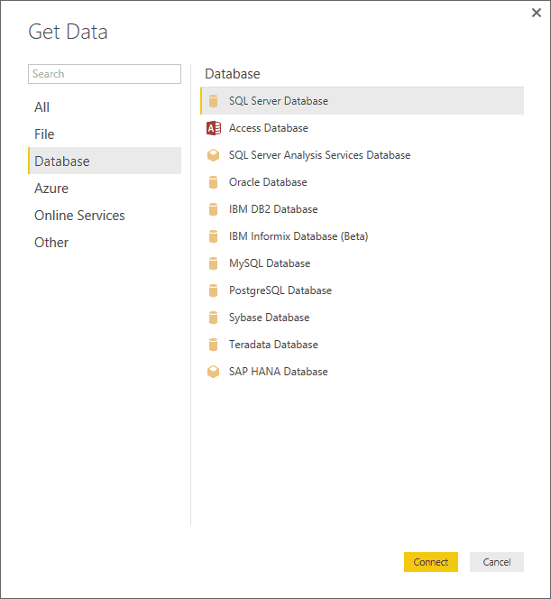
   Figure 1. The Get Data dialog

4. Click the ‘Connect’ button. The SQL Server Database dialog will appear.
5. Enter the server name in the ‘Server’ text box. This will be the name of your SQL Server or one of the SQL Server resources used by your organization.
6. Enter the database name; if you are using the sample data provided with this article, it will be CarSalesData.
7. Click ‘DirectQuery’ to connect live to the SQL Server database. The dialog will look like it does in Figure 2.

   

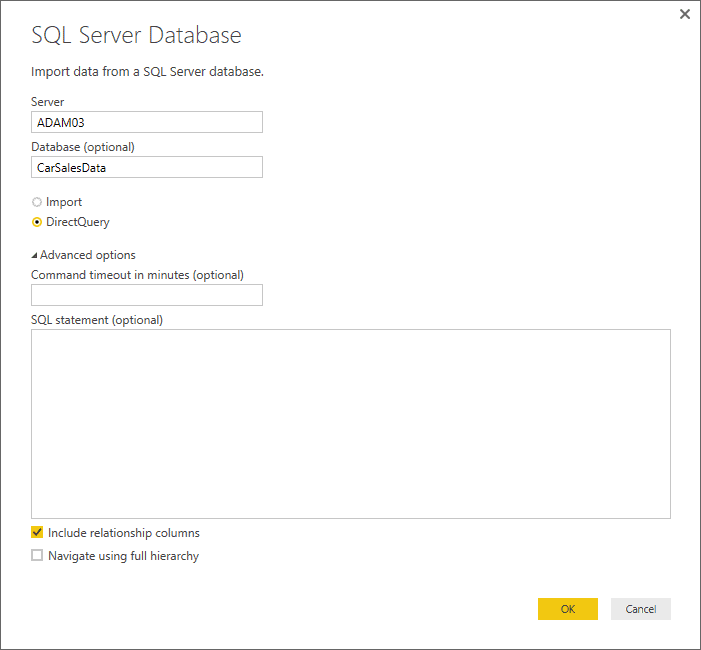
   Figure 2. The Microsoft SQL Database dialog

8. Click ‘OK’. The ‘Access a SQL Server Database’ dialog will appear. Assuming that you are authorized to use your Windows login to connect to the database, leave ‘Use my current credentials’ selected. The dialog will look like Figure 3.

   

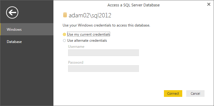
   Figure 3. The Access a SQL Server Database dialog

9. Click ‘Connect’. Power BI Desktop will connect to the server and will display the Navigator dialog containing all the tables and views in the database that you have permission to see on the server you selected. In some cases you might see a dialog saying that the data source does not support encryption. If you feel happy with an unencrypted connection then click the ‘OK’ button for this dialog.
10. Click on the check boxes for the Clients, Colors, Countries, Invoices, InvoiceLines and Stock tables. The data for the most recently selected data will appear on the right of the Navigator dialog. The Navigator window will look like Figure 4.

    

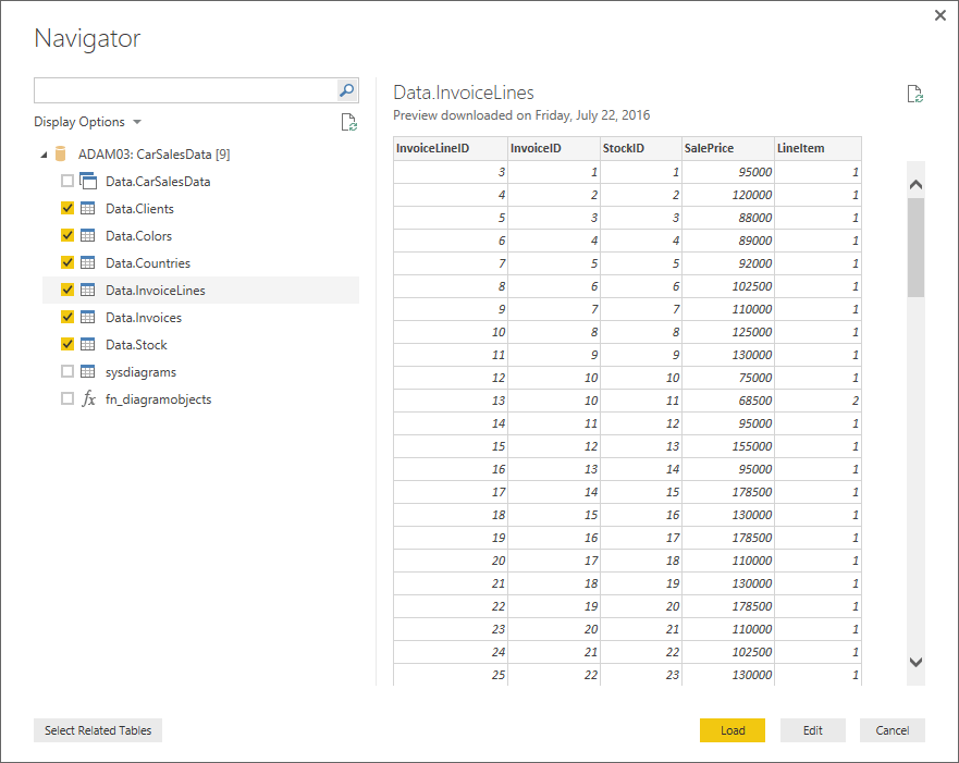
    Figure 4. The Navigator dialog when selecting multiple items

11. Click Load. The Power BI Desktop window will open and display the tables that you selected in the fields list of the Report window.

If you have had any experience of Power BI then you are probably thinking that this is a perfectly standard data load. You are indeed correct-because it is in many ways. The only major difference is that no data has been downloaded from the source database yet. So the data “load” was much faster than it would otherwise have been had you imported data.

Another difference-albeit a visual one-is that you can no longer see the Data view icon at the top left of the Power BI Desktop window. Only the Report and Relationships icons are visible. This is shown in Figure 5.

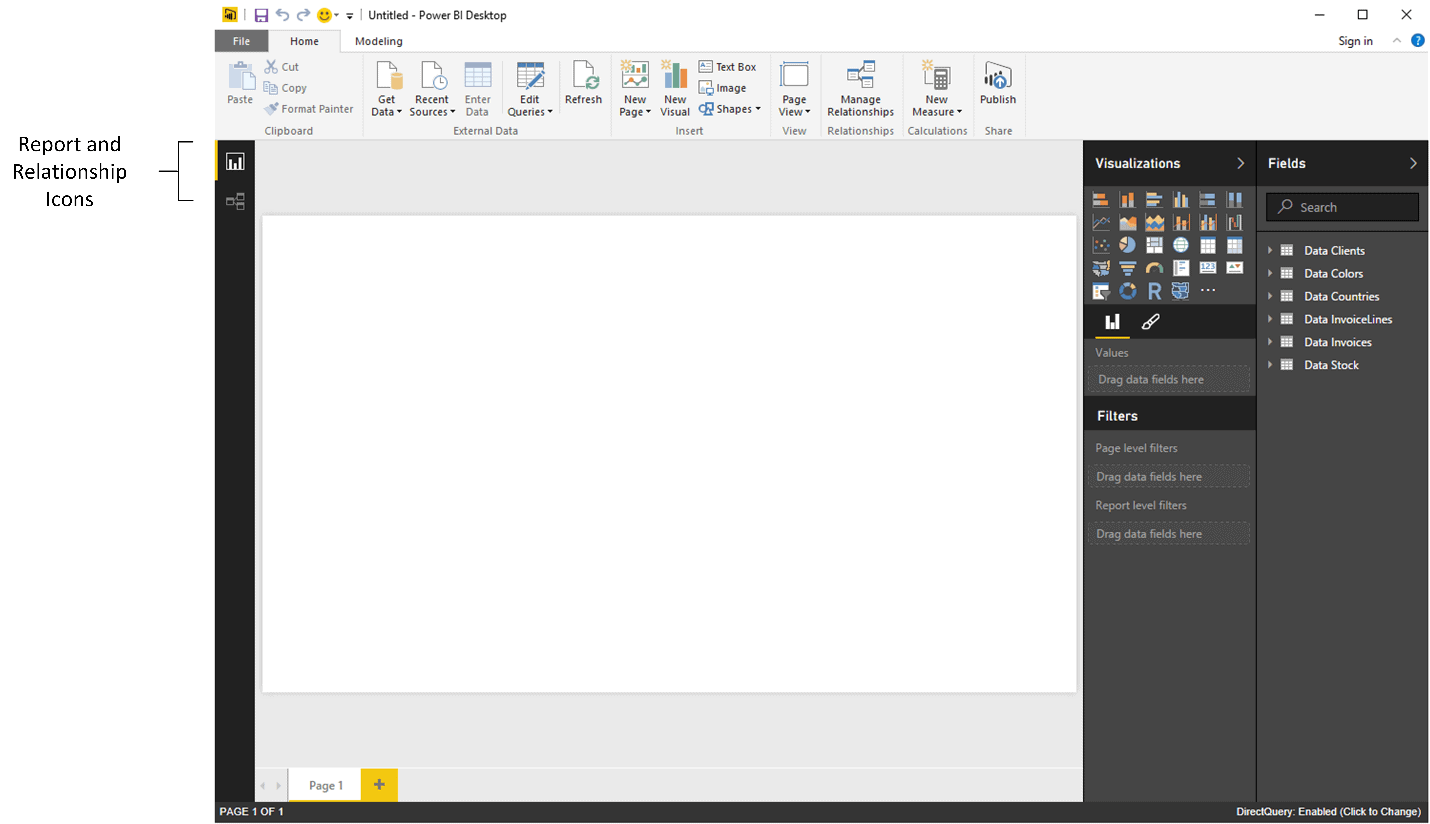
Figure 5. The view icons when DirectQuery is used

Connecting to the Source Data

Although I did not demonstrate it above, you can use all of the same techniques when using DirectQuery that you would use for a “classic” data load. This includes writing a custom SQL query to extract data or using the Power BI Navigator to search for tables in all the databases that you can access on a server.

Using the Source Data

Once the connection has been made, you can use any of the available fields in the source tables that you selected in order to create tables, matrices, charts and KPIs. All of the available visualization resources, as well as any third-part visuals that you have added, will work perfectly normally.

You might experience a short delay when creating a new visual in a dashboard that uses a direct connection. This is because Power BI Desktop is creating the query that is required to extract the requisite data,sending it to the server and ingesting the data that is returned. It follows that the time taken to return the data will depend on many factors including the server capacity and the current workload any available indexes that can be used. It will be faster to extract just a subset of the data than to download and compress an entire dataset.

As I have no wish to compete with Rob Sheldon’s excellent introductory article on Power BI Desktop (https://www.simple-talk.com/sql/reporting-services/working-with-sql-server-data-in-power-bi-desktop) I suggest that you consult this source for more information on how to create dashboards with Power BI Desktop. The only difference is that you can use DirectQuery when establishing a connection to the source data.

Editing Source Data

Using DirectQuery does not preclude you from availing yourself of all that the PowerBI Desktop Query Editor has to offer. So at step 7 in the data load process that you saw previously, you could just as easily have clicked ‘Edit’ and invoked the Query Editor. Or, as you will see now, you can return to the Query Editor from either the Reports or Relationship views and apply a wealth of data transformations to the source data when using DirectQuery.

For example, suppose that you want to remove a couple of columns from the Countries tables, as they contain data that cannot, or will not, be used in Power BI reports:

1. Click the Edit Queries button in the Home ribbon. The Query Editor window will open, looking like the one in Figure 6.

   

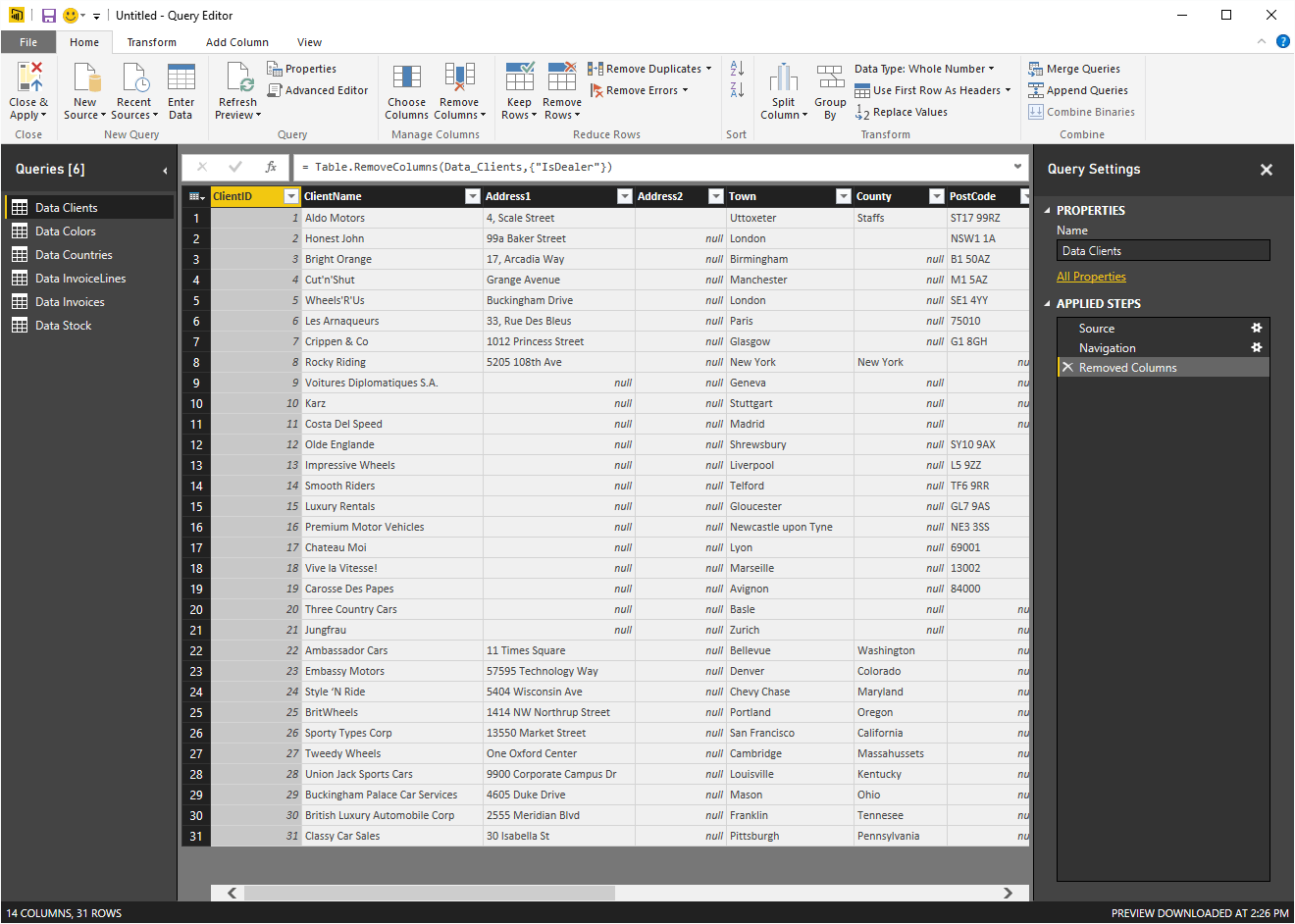
   Figure 6. The Power BI Desktop Query Editor window

2. Click on the ‘Data Countries’ table in the ‘Queries’ list on the left. The Countries data will be displayed.
3. Select the ‘CountryFlag’ and ‘CountryFlagURL’ fields.
4. In the ‘Home’ ribbon, click the ‘Remove Columns’ button.
5. Click ‘Close’ and ‘Apply’ to return to Power BI Desktop.

Once back in Power BI Desktop you will see that, if you expand the Countries table, the two columns that you just removed in the Query Editor are no longer available to users.

This was, inevitably, a trivial example of the way that source data can be modified using the PowerBI Desktop Query Editor. However the point is that using DirectQuery does not bypass the Query editor. All of its ETL potential is still available to help you transform and shape your source data. This can range from renaming a couple of columns to transforming a relational data model into a logical data vault using intermediate queries and aggregations.

Creating a Data Model

Data modelling is another key aspect of Power BI Desktop that remains available when using DirectQuery and a database source. So, even if relationships between tables in the source data have not been recognized (or if they do not exist), you can always add them for the benefit of your Power BI data model.

To join the Colours table to the SalesData table:

1. Drag the ColorID field from the Stock table over the ColorID field in the Colors table as shown in Figure 7.

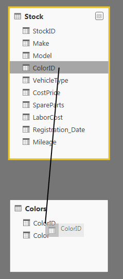
Figure 7. A table relationship

This is all that you have to do. The two tables are now joined and the data from both tables can be used meaningfully in reports and dashboards.

Once again this is a simple example. Yet the principle holds that you can extend the data model from a DirectQuery link just as you can when downloading data. It took less than a minute to create the data model that you can see in Figure 8 using the source data tables that were in the sample database.

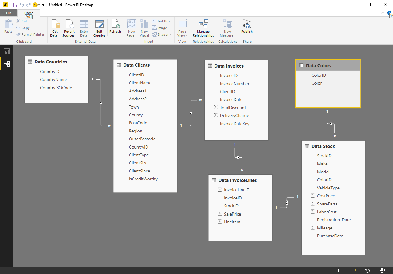
Figure 8. A data model created in Power BI Desktop using a direct connection

Adding Columns

Let’s now add a calculation to the Stock table. More precisely, I will assume that our Power BI Desktop visualizations will frequently need to display the figure for the direct costs relating to all vehicles purchased, which I will define as being the purchase price plus any related costs. This is, of course, an extremely simple modification, but I am including it as an introduction to basic data modelling in Power BI for any readers who have not yet experimented with these aspects of the product.

1. In Data View select the Stock table.
2. Click ‘New Column’ in the ‘Modeling’ ribbon.
3. Replace the word ‘Column’ in the formula bar with the word ‘Direct Costs’ (notice that there is a space, because column names can contain spaces).
4. To the right of the equals sign, enter a left-square-bracket [. The list of the fields available in the Stock table will appear in the formula bar.
5. Type the first few characters of the column that you want to reference—CostPrice in this example. The more characters you type, the fewer columns will be displayed in the list.
6. Click on the column name. It will appear in the formula bar (including the right bracket).
7. Enter the minus sign.
8. Enter a left parenthesis.
9. Enter a left-square-bracket ‘[‘, and select the column SpareParts.
10. Enter a plus.
11. Enter a left-square-bracket ‘[‘, and select the column LaborCost.
12. Enter a right parenthesis. This corresponds to the left parenthesis before the SpareParts field. The formula should read
    1	DirectCosts = [CostPrice] - ([SpareParts] + [LaborCost])

13. Click the tick box in the formula bar (or press Enter) and the new column will be created. It will also appear as a new field in the ‘Fields’ list for this table.

As you can see, using arithmetic in calculated columns in Power BI Desktop is almost the same as using calculating cells in Excel. If anything it is easier because you do not have to copy the formula down over hundreds or even thousands of rows as the formula will automatically be applied to every row in the table.

Adding Measures

Some data, especially when sourced from transactional systems, is difficult for the layperson to understand. So you could be asked to extend the source data with specific metrics. Users, and this means the target audience for your reports and dashboards, do not like anomalies or apparent contradictions. So you have to ensure that the data that they see is visually coherent. This is especially true when displaying tables and matrices with subtotals and grand totals. This requires applying a little DAX to the data.

One technique that can help you here is to use the Allselected() function. This will only apply any filters that have been added (either at Report-, Page- or Visualization-level or as slicers or cross-filters from other visuals) without you having to specify the fields that you do not want to filter as you did in the previous examples.

Here is a measure – SalesPercentage – that uses the Allselected() function as the filter for the Calculate() function that returns the percentage total of an element relative to the grand total.

If you take a look at Figure 9 you will see that the subtotals for the sales percentage (and indeed the grand total) are accurate, despite the fact that the country USA is selected in a slicer and the year 2014 in a filter.

Figure 9. Using the Allselected() Function to calculate a percentage per attribute per group

The Allselected() function says to DAX “don’t filter on any filters applied by the user, whatever the technique used to apply them”. This can make creating percentage totals much easier, as this function removes the need to create highly specific measures that are tied to specific types of calculation.

In a simple example you have seen that you can add DAX formulas to directly queried data sourced from an SQL Server database. Any measures created this way will be recalculated on the fly as required. Suddenly considerable horizons for real-time data analysis have opened up-not to mention a really good reason to get proficient in DAX.

So now that we have confirmed that DirectQuery works pretty much like any other data source connection, let’s take a quick look at some variations on a theme. This will include connection to data warehouses (both SSAS dimensional and SSAS tabular) as well as connecting to SQL Server in-memory tables.

DirectQuery and Classic SSAS

To continue this whirlwind tour, I propose to use Power BI Desktop as an analytical interface for a “classic” SQL Server Analysis Services (SSAS) cube. There are, after all, hundreds of thousands, and possibly millions of these analytics solutions operational throughout the world. Consequently Power BI should be able to link to the massive amounts of data that they contain and allow users to slice, dice and otherwise delve into the information that they hold.

If you do not have an SSAS cube to hand, then you can always restore the small SSAS 2014 Analysis Services database that is provided with the samples for this article.

1. Open a new Power BI Desktop Application.
2. In the Power BI Desktop ribbon, click the small triangle at the bottom of the Get Data button, then click SQL Server. The SQL Server Database dialog will appear.
3. Enter the server name in the Server text box. This will be the name of your SQL Server or one of the SQL Server resources used by your organization.
4. Enter the database name if you have it.
5. Ensure that the Connect Live button is selected. The connection dialog will look like Figure 10.

   

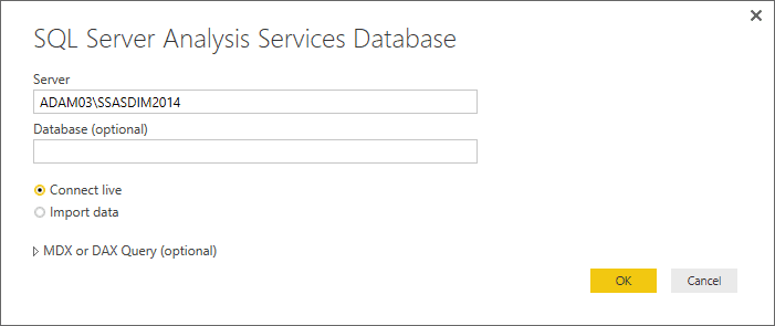
   Figure 10. Connecting to an SSAS data warehouse

6. Click ‘OK’. The Navigator dialog will appear rather like the one that is shown in Figure 11.

   

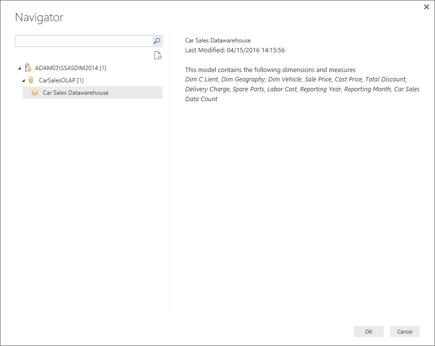
   Figure 11. The Navigator Dialog for a direct connection to an SSAS data warehouse

7. Click ‘OK’. The Power BI Desktop Report view will appear as shown in Figure 12.

   

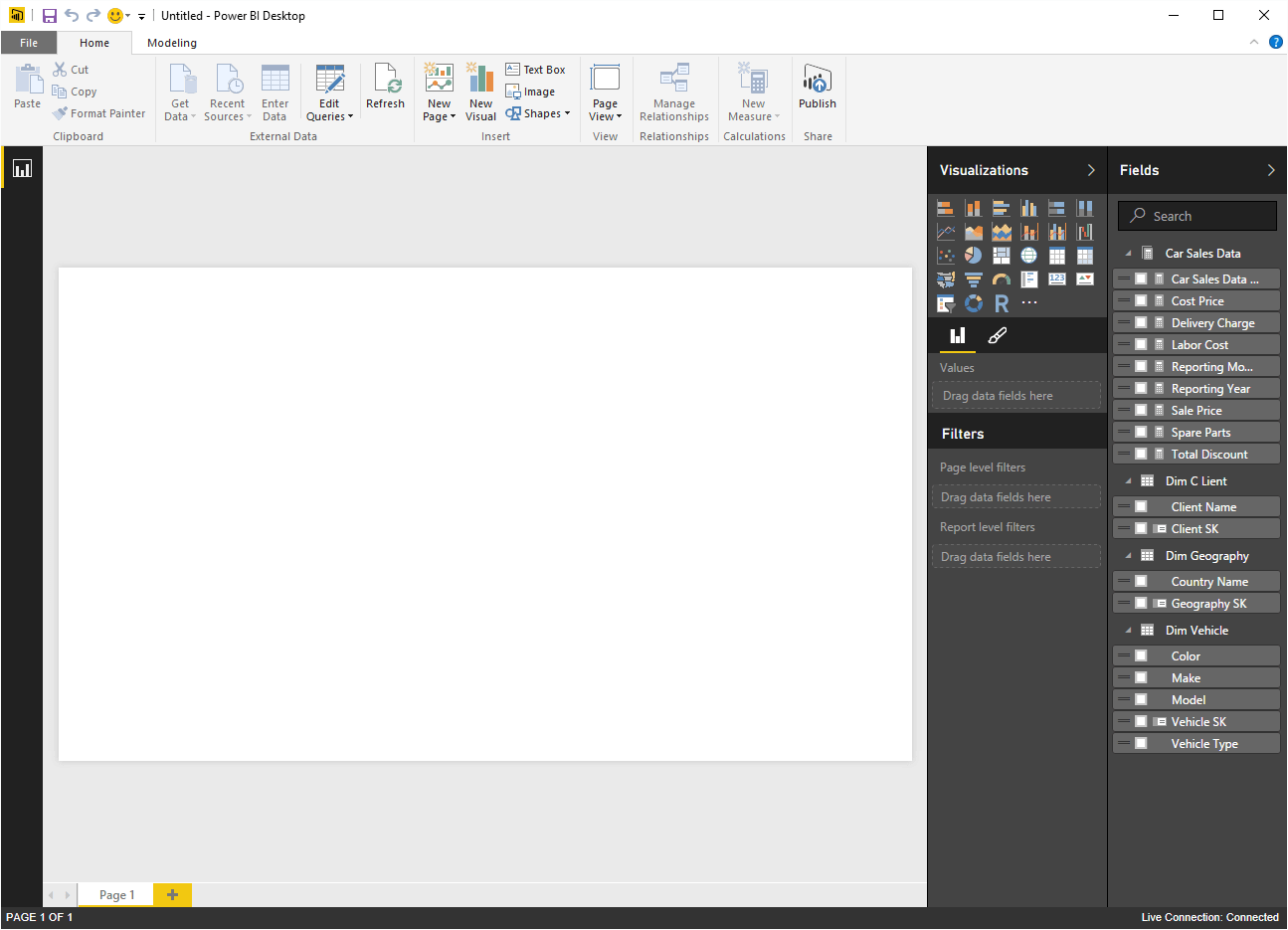
   Figure 12. The Power BI Desktop Report view for a direct connection to an SSAS data warehouse

While establishing the connection is truly simple, a few comments are necessary at this stage.

• When you use DirectQuery to connect to a classic SSAS instance you are exposing the entire cube to the user. You cannot select a specific subset of attributes and measures – as you can see in Figure 11.
• You cannot hide or remove metrics or attributes in Power BI Desktop.
• You can, fortunately see and drill into existing hierarchies in the cube.
• You cannot add calculated columns or measures. As you can see in Figure 12, the New Measures button is greyed out – and the context (or right-click) menu will not display the option to add calculated columns or measures.
• You cannot modify the data model in any way. As you can also see in Figure 12, only the Report View icon is available for an SSAS DirectQuery connection in Power BI Desktop.
• You cannot modify the source query. Clicking the Edit Queries button in the Home ribbon will only display the following dialog

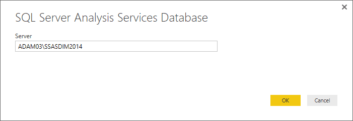
Figure 13. The Power BI Desktop Edit Queries dialog for a direct connection to an SSAS data warehouse

Clicking ‘OK’ from this dialog will simply return you to the Navigator dialog that you can see in Figure 11.

As was the case with a direct connection to a SQL Server relational database, you will probably experience a slight delay when adding or modifying a visual in a dashboard. Once again this is because Power BI Desktop is creating and sending the necessary query to the source server and returning only the required data. Inevitably, the time taken to return the data will depend on the size and optimization of the SSAS cube and the underlying hardware.

A direct connection to an SSAS cube does have a few limitations. However to be fair there are also a few limitations when you connect to an SSAS cube and download the data into the local in-memory model.

Firstly, you need to remember that when you connect Power BI Desktop to an SSAS cube and download the data you have to select all the measures and attributes that you require, as shown in Figure 14.

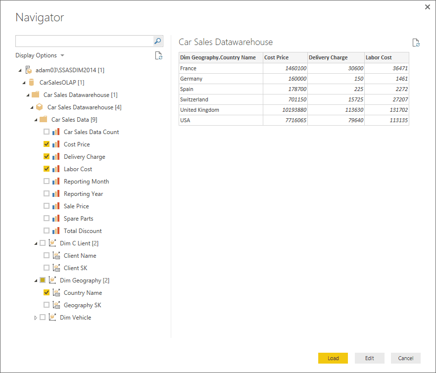
Figure 14. Selecting attributes and measures when connecting Power BI Desktop to an SSAS cube

Moreover, not only do you have to state explicitly and individually which attributes and measures you want to use, you are then presented in Power BI with a single flattened table. This is shown in Figure 15.

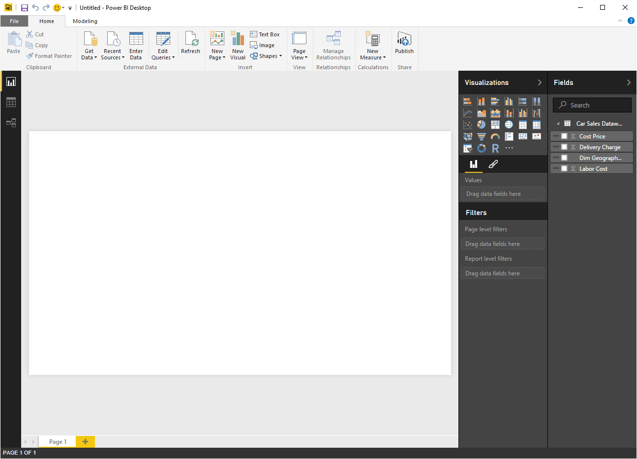
Figure 15. The attributes and measures in Power BI Desktop from an SSAS cube

And finally, when connecting Power BI Desktop to an SSAS cube and selecting even a small subset of the available data you can easily end up with a huge dataset that takes an extremely long time to download and compress into the local in-memory model. So both connection types have their advantages and disadvantages when using SSAS as the source of the analytical data.

Direct Query and In-Memory Data Sources

As virtually the only drawback so far to using DirectQuery has been the time taken to return data from large datasets the next step is clearly to try and speed up the data query and transfer. The most obvious solution is to take advantage of all the efforts that Microsoft has made to enable in-memory solutions. For starters, let’s see if DirectQuery will work with a SQL Server 2014 database where the table(s) are defined as in-memory OLTP tables.

If you do not have any in-memory data tables to hand, you can always use the sample database CarSalesMemoryBased that is supplied with the downloadable files that accompany this article.

If you have not yet used in-memory tables with SQL Server, then remember that you will need to prepare the database for their use. To save you digging for information, the basic code to enable a SQL Server 2014 or 2016 database for in-memory tables will require code like the following:

All the tables in this database are all defined using the following option:

As an example, the Clients table is defined like this:

With this in mind, let’s try and connect Power BI Desktop to the tables in this database, pretty much as we did for the first DirectQuery example in this article.

1. In a new Power BI Desktop window click Get Data and select SQL Server database.
2. Enter the Server name and the database name (CarSalesMemoryBased in the sample data) in the SQL Server Database connection dialog.
3. Select DirectQuery.
4. Click ‘OK’.
5. Select all the tables in the database as you did previously.
6. Click Load.

All in all the process is identical to the previous one for a relational database. In fact the process is so similar that you can refer to all the screenshots in figures 1 through 4 above when connecting to in-memory tables. So what are the differences? Well, as far as I can see there are none at all. A direct connection to a set of in-memory tables (or even a mixture of in-memory and disk-based tables) is, to all intents and purposes identical to a connection to a standard SQL Server database. You can alter the data model, add measures and calculated columns – indeed treat data from in-memory tables just as you would any other relational data source.

So what differences are there? Inevitably there is one major factor that you will notice immediately when querying data – speed. As you would expect, querying data from the server’s memory is considerably faster. Clearly you will not see much of a difference when using a small sample dataset such as the one supplied with this article. However if you are fortunate enough to have a large dataset in one or more in-memory tables (which, by definition, is on a server that has a decent amount of memory) you are likely to experience the difference instantaneously.

DirectQuery and SSAS Tabular

In the real world, however, you are probably unlikely to be querying in-memory tables for large datasets simply because placing large datasets in memory is a costly business. It is more likely that an in-memory solution will be using a technology such as SSAS tabular. So the next step is to see how (and indeed if) you can connect Power BI Desktop to an SQL Server Analysis Services tabular data warehouse.

1. In a new Power BI Desktop window click Get Data and select database and SQL Server Analysis Services Database.
2. Enter the Server name and the database name (CarSalesTabular in the sample data) in the SQL Server Database connection dialog..
3. Select ‘ConnectLive’. The dialog (if you are using the sample SSAS tabular database supplied with this article) will look like Figure 16.

   

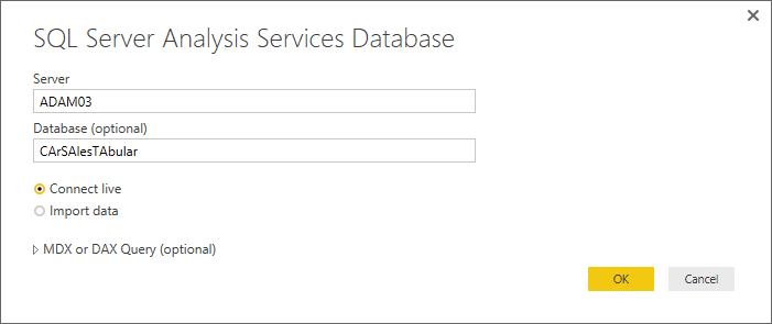
   Figure 16. Direct Connection to an SSAS tabular data warehouse

4. Click ‘OK’.
5. Select the tabular data warehouse from the Navigator dialog. In this example it is called Model, as you can see in Figure 17.

   

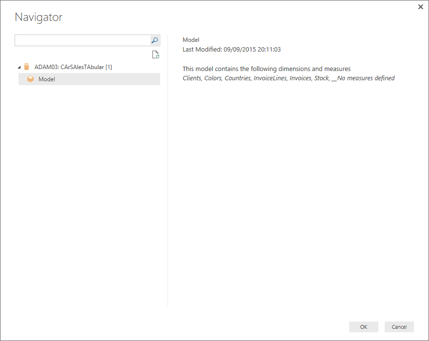
   Figure 17. Selecting the database in a SSAS tabular data warehouse

6. Click ‘OK’. You will connect to the data and see the Power BI Desktop View Pane that is shown in Figure 18.

   

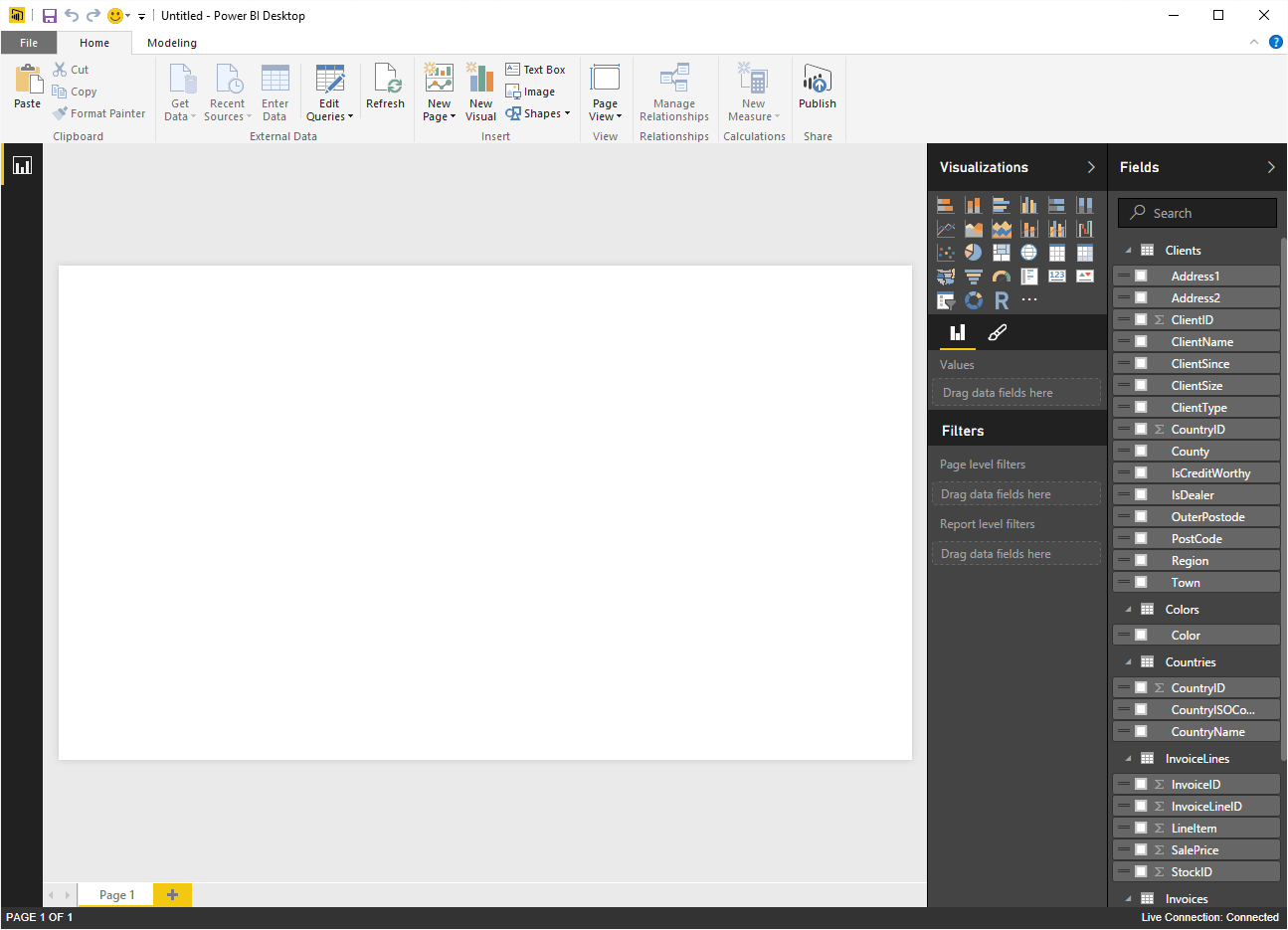
   Figure 18. Power BI Desktop using a Direct Connection to an SSAS tabular data warehouse

As you can see in Figure 18 a direct connection to an SSAS tabular data warehouse:

• Does not let you access the data model (the only available display icon is the Report icon).
• Does not let you add measures or calculated columns (the New Measure button is greyed out).
• Does not let you hide tables or fields.

So, put bluntly, using an in-memory connection to an SSAS Tabular data warehouse presumes that the source data has been comprehensively modelled before being deployed and that all the measures and attributes are available for users.

Yet any potentially negative points soon pale into insignificance when you get down to the business of analyzing the source data. The fact that the data is not downloaded into the local data model, coupled with the source data itself being both compressed and stored in-memory results in extremely rapid response times. Of course, just how fast you are able to see visuals when you create them will depend on a significant set of infrastructure and networking factors. Nonetheless the key point to make is that response times will make a quantum leap from the painful to the impressive when making a direct connection to an SSAS tabular data warehouse.

I feel that this point cannot be made too forcefully. When you connect Power BI to SSAS tabular data warehouse you have a technology marriage made in silicon heaven. In fact, after a few minutes use you will probably never want to use any other front end to access data stored in this platform. Of course, you have to ensure that the back-end data model is complete and contains all the data and metrics that you and your fellow users will need. But isn’t that what we call BI anyway?

Direct Query and In-Memory Analytics

While writing this article I – like so many others – am eagerly experimenting with SQL Server 2016. One of the many facets of this release that is of relevance to the discussion on DirectQuery is the potential for in-memory analytics. What this means is that SQL Server 2016 offers the possibility of using tables in memory that use the kinds of structures (columnar storage and compression) that suit analytic workloads, but in a relational database.

When using an SQL 2016 instance the database was enabled for in-memory data, just as was the case for a SQL Server 2014 instance. Then the tables were defined to enable clustered columnstore in-memory indexes. As an example, the DDL for the Colors table looks like this:

Once all the data tables have been created – and the data loaded – you can set up a direct connection from Power BI Desktop to the database. This process is identical to the very first example in this article or the previous example for connecting to in-memory tables. There are absolutely no differences. A DirectQuery connection to columnstore in-memory tables will let you carry out all the standard Power BI operations such as (and this list is far from exhaustive):

• Filter source data
• Modify data types
• Rename tables and columns
• Define and extend the data model
• Add calculated columns and metrics
• Create hierarchies
• And pretty much everything else that Power BI can do

So whatever the database storage technique, Power BI will read the data in exactly the same way, and allow you to filter, model and enhance the data with metrics and calculated columns just as you would for a classic SQL database. Only you now have real-time analytics on an OLAP database with vastly reduced refresh times using a simple and immensely powerful user interface.

That last sentence merits rereading to grasp the power that you have just unlocked. You could now no longer need to extract and process data from an OLAP system into a data warehouse, and can shape and extend the analytical model to present users with a comprehensible dataset that contains only the data that they need yet can contain added metrics and structured hierarchies of attributes. Indeed, Power BI Desktop Query Editor will let you overlay a completely difficult logical layer over an existing in-memory relational data structure – as you will see in an upcoming article on Simple-Talk.

DirectQuery and PowerBI.Com

Reports created using DirectQuery can be published to the Power BI Service You will need to set up a Gateway to allow data refresh from on-premises data. However this is a separate subject and cannot reasonably be handled here.

Conclusions

In this article you have seen some of the data sources that allow you to connect directly when using Power BI as a data analysis and visualization tool. Above all you have seen that you can connect to the data just as you would for a “standard” Power BI connection, and that – depending on the data source – you can modify and extend the data to support in-depth and expressive analytics.

There are, arguably, three key benefits to using DirectQuery as a source of data:

• DirectQuery lets you build reports based on extremely large datasets, this is particularly true in the case of huge tables where it would simply not be practical to import all of the data
• Underlying data changes can necessitate data being refreshed frequently. It follows that for some reports, a requirement for up to the minute data can require massive data transfers, making re-importing data not a practical solution. By contrast, DirectQuery reports always use current data, and the hard work is carried out where it should be done – on the server.
• When you re-query data that has been recently requested by Power BI the application will re-use existing data to avoid swamping the server with pointless requests for data.

Nonetheless, there are a few drawbacks to using DirectQuery. They include the following:

• All tables must come from a single database. There is simply no way of combining data from multiple sources yet. Of course, you can always see if it is possible to create a single database that contains views over linked databases so that Power BI Desktop can obtain the source data from a single data connection that masks the underlying cross-database links.
• If the Query Editor query is overly complex an error will occur. To remedy any error you might have to import the data instead of using DirectQuery.
• Relationship filtering is limited to a single direction, rather than both directions.
• By default, a few limitations are placed on the DAX expressions that are allowed in measures. Unfortunately these can only be discovered the hard way, as you encounter error messages when Power BI Desktop queries the data source.
• There is no easy way to convert a Power BI Desktop file from DirectQuery to a connection that downloads the data to the local data model. You simply have to create a duplicate file with a “classic” connection. This will mean exporting and/or recreating any measures and calculated columns that you have added to the DirectQuery dashboard.

Inevitably, establishing a direct connection to a data source will not resolve every challenge. Above all it will not remove the requirement to apply careful thought to the way that you handle your analytic data. So you will probably still need to:

• Only select the source data that you really need, this can mean
  • Filter the data (where possible) using custom SQL, MDX or DAX queries to ensure that only essential data is used by Power BI Desktop.
  • Select only the objects (again, where this is possible) that you really need to use
• Give careful consideration to the structure of the data that you are accessing. Complex data structures will, inevitably, lead to slower output.
• Where possible, think of end-users when developing Power BI solutions for less technical people. This can mean that, when using relational sources, you might need to hide tables and fields and add any necessary hierarchies and metrics – so that a more operational (not to say “raw”) data source becomes comprehensible and useable by non-technical staff.

There is, self-evidently, a lot more that could be said about using direct connections to the data sources that support this kind of access. There is simply not enough space here to cover all the possibilities or data sources. However I hope that I have been able to convince you that there are many circumstances where a direct connection to a data source is worth any extra effort. Specifically the vastly increased speed with which you can create, modify and refresh reports based on extremely large datasets using Power BI Desktop should prove to be an essential motivating factor. When the dust has settled this simply means faster, cleaner and more impressive analysis.