Part II : Equivalent Solutions in Functional Programming – Scala

Part I of this two-part series presented the series problem then solved it in SQL Server. However, this was a simulation meant to provide the following: result sets against which the actual software can verify; and a query execution plan that can serve as a pattern for the actual software design. In this second of the series, components from the former guide the software development, which will be done in functional programming – specifically, Scala.

Scala is not a CLR language, so I don’t expect you to know it. Therefore, the article starts with just enough background in functional programming and Scala to follow the discussion. You do, though, need some experience in any imperative or functional language so that structures such as lists, sets, and maps are familiar.

Declarative programming is a major theme in this series. You already know the style from work done in (T-)SQL DML. If you are unfamiliar with functional programming, then consider this article a voyage into a foreign paradigm in which concise and elegant logic describes transformations over immutable data. Keep in mind that there is much more to functional programming than is presented here – emphasis, again, is its declarative nature.

The Scala file and its executable (not included), runnable in PowerShell, plus all project files are available in the download.

Functional programming: Basics in Scala

This cursory look into functional programming (FP) starts with relevant terms and concepts, and I’ll add more later as the discussion progresses. The second subtopic examines the anonymous function, and the third, map functions. Return to this section as needed or skip it if you know Scala.

Terminology and concepts

At the highest level, functional programming is about composing operations over immutable data. Operations are functions written declaratively – i.e., in concise logic that describe transformations. Functions do not alter object or program state; they only compute results. Contrast this with the imperative programming style, such as object-oriented programming (OOP), in which lower-level steps delineated in order in sequences and loops and branches can change program state.

In FP, functions are pure, meaning that they have no side effects such as reading from or writing to data sources or mutating data in place. As a result, given the same input values, a pure function always returns the same output value. Furthermore, they always return a usable value, never a void (Unit in Scala), which signifies that the method is invoked to produce a side effect(s). In the solution’s sections, I’ll isolate all pure functions in one place.

(C# and perhaps all languages allow writing pure functions. FP takes it much further.)

Here are some Scala-specific keywords you will see in explanations and code:

• trait. Roughly analogous to an interface in OOP.
• def. A named method.
• val. A variable that can’t be reassigned to a different value.
• type. A user-defined alias, possibly parameterized, for a data structure or function
• object. A one-instance class whose members are (therefore) all static (one copy only). Can be standalone or companion to a trait or class when they share the same name. The latter type is used in the code.

Finally, and critically, FP functions are first-class values, meaning they can appear anywhere a type-referencing variable can.

Next is an important kind of function.

The Anonymous Function

An anonymous function is any that is not a named, reusable method – i.e, not introduced with the keyword def in Scala. It is also known as a function literal, and more universally, as a lambda expression. I’ll use anonymous function and lambda interchangeably. The arrow symbol => separates the bound parameters, if any, from the computation. Bound variable names are arbitrary.

Figure 1. A Scala anonymous function with two bound parameters

This basic example next shows a variable bound to an anonymous function and its invocation. Variable timesThree represents an unnamed function of type Int (integer) to Int – left of = – that is defined as taking an Int argument x and returning a transformed Int value.

Figure 2. One of several ways to define and use an anonymous function

Colons indicate variable types and return type.

A higher-order function takes a function(s) as a parameter(s) and/or returns a function. Thus, an anonymous function, a variable such as timesThree, or a named method could all be arguments.

Figure 3. A well-known kind of higher-order function

Higher-order method composeInt takes two function parameters and does a common operation. Without providing the x value (3) argument, the return is a lambda as was echoed to screen (Int => Int).

NOTE: These examples were done in PowerShell. To try this on Windows, you must set up the Java JDK and Scala. Some websites, though, let you enter and run Scala code in a browser – just learn the println() command.

Two important higher-order functions are next.

Map functions

A polymorphic function is one parameterized by type(s), allowing methods to be written generically, independent of instantiating type. A type can be the return type or type held by the returned containing object, and/or type of a parameter(s).

Known by varying names in possibly all FP languages are Scala’s polymorphic functions map() and flatMap().

Figure 4. A higher-order polymorphic function for sequence collections

Type parameters in Scala are in square brackets. The Seq trait is a supertype for sequence collections such as list and vector.

Part I showed that declarative T-SQL code could be translated into a loop implementation by the query optimizer. In a similar vein, map() abstracts looping over all collection elements, applying the polymorphic function ‘f’ parameter to each element. This is the result:

The original collection is unchanged; a new collection of the same class – in this example, a Seq subclass – holding the transformed elements of type B is returned.

Type B may or not be the same as type A, held in the original collection.

The map() can be chained with other map() calls and other operations but is not suited to nest another map() to simulate a nested loops pattern. This requires a more powerful form of map function.

Figure 5. The flatMap function signature

The IterableOnce trait is a more general base for all traversable data structures, as it covers the sequences in examples here as well as Sets and Maps and some non-collection types as well.

The background ends here. You will see maps and other higher-order functions in the solutions.

Solution space: IceCream trait

Having the download file IceCream_client.scala open aids the discussion. The commented code file also has many features and tests I won’t cover in this article. Make sure you have the latest version of the file, as it has changed since the release of the first article.

Recall the T-SQL query plan from Part I:

Figure 6. Query plan from Section ‘Query Rewrite II’

The subtopic covers translating the plan into methods and index simulators in Scala.

Mirroring the T-SQL Query Plan

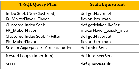
The following table shows the mapping from query plan items – the T-SQL blueprint above – to Scala pure functions and index simulators. Both will be covered in detail in subsequent topics.

Figure 7. Query plan to Scala mapping

Notice that there isn’t a precise correspondence from T-SQL to Scala objects. In rows two and three, the clustered index seeks, which use the primary key, reflect to different Scala methods and index simulators. In rows one and three, two different index seek types and index usage map to the same Scala method and index simulator.

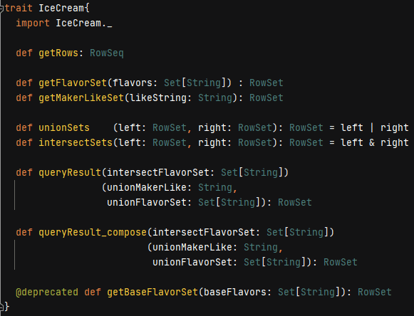
Figure 8. Trait as client interface

The IceCream trait in the figure above serves as the Scala client interface of available methods.. Two are defined in the trait, and the rest are abstract. Additional methods, some of which to be discussed, are documented in the download Scala file.

Since most relational tables have primary keys, they are sets, whether well-normalized (redundancy-free) or not. The query plan operators in the rewrite produce and work with denormalized sets of rows. In parallel, almost all trait functions return RowSets and have Set or RowSet parameters. This is by design. RowSet – meant to be intuitively named – is defined anon.

Client software now needs a way to create the object that implements the IceCream contract.

Solution space: IceCream companion object

Some data types in the trait are user-defined aliases from the companion object.

Figure 9. Type aliases and factory method

A Row is a three-tuple of strings representing (Maker, Flavor, Base Flavor). Types RowSeq and RowSet, then, are sequence and set parameterized data types holding the tuples. Tuple components are referenced with _x position notation, where x is 1,2,3…

The apply() function in companion objects has special meaning: it is a factory method clients use for creating the implementing object. In the IceCream project, the companion creates its own private class, passing it the RowSeq data, and returns the trait interface. This hidden implementation/separation of concerns style is a common design paradigm.

The object’s private class IceCreamImpl extends – roughly, inherits – the trait and encapsulates the resources for doing all data transformations.

Solution Space: IceCream Implementation

I’ll now broaden the meaning of ‘blueprint’ to include the query plan (Figure 6), its mapping to Scala equivalents (Figure 7), and the IceCream trait interface (Figure 8). Hidden class IceCreamImpl now has its pattern.

Figure 10. Implementation class’ initial data and trait extension

The rows in the parameter list is the OS file data, and keyword extends is analogous to OOP inheritance but follows different rules (not covered).

The two subtopics cover building the index simulators and realizing the interface. All code is within class IceCreamImpl.

Class construction: Index creation

T-SQL indexes (roughly) translate to key-value (k-v) pairs, which equate to the Map data structure. I’ve set up keys and values using a trait and case classes. A trait can be used solely for grouping related items, and a case class, for purposes here, is a class created without keyword ‘new’ and whose constructor parameters are default public.

Figure 11. Structures used by index simulators

From the blueprint, primary key index PK_MakerFlavor has a compound key (Maker, Flavor) to which MF corresponds. In figure next, the Map is built from the initial data using several map functions:

Figure 12. The primary key equivalent

In the first code line (rows.groupMap…), in its first argument list (currying – not covered), the Map key is set to the composite key equivalent MF for every element in list rows. Put more explicitly: function groupMap iterates over every three-tuple (Maker, Flavor, Base Flavor) in the rows sequence of initial data, binding local variable row to each tuple at each pass. The entire argument – ((row: Row) => …) – is a lambda.

The second argument list sets the k-v value to the Base Flavor (shorthand tuple access _._3, also a lambda). The result is a Seq[String], where String is base flavor. This, though, is misleading. Per the business rules (Part I), a single value, not an ordered sequence of values, is correct and clearer. This is done in the next two lines.

On the newly generated Map, its flatMap() – essentially, the outer loop – iterates over every k-v pair. The nested map() – inner loop – translates and returns each one-row sequence (kv._2) of base flavors into the k-v value. A k-v pair in Map is represented as (k -> v).

If you’ve never worked with functional programming, I hope you are reading for the gist of it and appreciate its compactness and elegance (among other benefits).

The IX_MakerFlavor_Flavor covering index simulator can be built from this primary key simulator:

Figure 13. The covering index equivalent

This time, again by the business rules, a sequence (list) of case class BM is correct, as sample output from both Map structures shows:

Figure 14. Sample equivalent rows from primary key and covering index simulators

The covering index simulator flavor_bm_map restructures the data in the primary key simulator makerFlavor_baseF_map exactly as it happened in the database.

Serving the interface

For brevity, I won’t cover the entire trait interface – just enough to explore using the indexes and deriving solutions. Refer to T-SQL to Scala mapping Figure 7.

Figure 15. Simulating index seeks

Method getFlavorSet is invoked to emulate two different T-SQL query plan operators using index seeks over the IX_MakerFlavor_Flavor and PK_MakerFlavor indexes (rows 1 and 3). The former restricts on Mint, Coffee, Vanilla and the latter, Vanilla solely, as given in the flavors parameter.

Method withFilter is a non-strict filter, meaning – in usage here – that it doesn’t produce an intermediate set that must be garbage collected but rather restricts the flatMap domain during its traversal of elements. Its lambda argument simply eliminates any flavor not recognized as a key in flavor_bm_map rather than throwing or handling an exception.

The flatMap iterates over every recognized flavor. The flavor_bm_map(flavor) operation returns the list of BM (base flavor, maker) case classes – the value in the k-v – and the map function takes each to form an individual Row.

Figure 16. Query result over three flavors

Method getMakerLikeSet corresponds to the upper Clustered Index Seek branch in the lower input to Nested Loops (row 2). The seek is done on the primary key index but is inefficient as its Predicate must tease apart the maker name. The method equivalent is worse.

Figure 17. The method finds all ‘Creamery’ makers (suboptimal)

The like argument trivially is ‘Creamery’. For every k-v key in the primary index simulator, the algorithm filters out all makers who aren’t ‘Creamery’ using a non-interface named method (not shown) rather than a lambda. (Without elaboration, a more optimal version is possible but involved.)

Deprecated function getBaseFlavorSet uses a third covering index simulator having base flavor as key. The first article proved why this index is not desired; here, as in the T-SQL, usage produces four rows to be culled later instead of the desired two. This was also proved in the Scala test run.

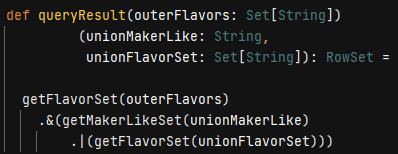
All needed methods and resources are now in place for IceCreamImpl to solve the series problem. Here is the first of two solutions:

Figure 18. Equivalent to T-SQL query rewrite II (final form)

The first parameter outerFlavors contains the three flavors as discussed; the second, Creamery; and the third, Vanilla. The first invocation of getFlavorSet mimics the query plan outer input to Nested Loops. This set of three-tuple rows intersects (‘&’) with the rows simulating the inner input, thereby paralleling the Nested Loops’ Inner Join logical operation. The call to getMakerLikeSet retrieves the Creamery rows and does a union (‘|’) with the second invocation of the getFlavorSet. The union mirrors the Stream Aggregate ← Concatenation operators.

The second, equivalent solution, is more function composition style.

Figure 19. Solution in function composition

The blueprint has been realized in software. All that is left is to verify the result:

Figure 20. Software and T-SQL yield the same result set

The Client

Programming side effects include I/O, and these are limited exclusively to the client, which consumes the IceCream trait and companion object. The client reads the data from the OS file, packages it for consumption by the factory method in the companion, and invokes the pure functions in the trait, printing results to screen. For brevity, here is a snippet from the call to apply():

Figure 21. Transforming the OS file data for IceCream factory method apply()

Variable v holds the data from the .csv file as a sequence of strings, and the tail function skips past the (Maker, Flavor, BaseFlavor) header. The first map() transforms each line in the sequence (Seq[String]) to an array size three of strings (Array[String]). A second map() chains to the first to turn each array into a three-tuple.

In Conclusion

This second and last article in the series gave a condensed background in functional programming and Scala. This included higher-order, pure, and map functions and lambda arguments. All data transformations were done using these constructs, plus a non-strict filter method. In good functional programming style, all coding was declarative: no low-level control flow statements were written.

The notion of blueprint was widened, first by a translation grid that mapped T-SQL query plan operators and indexes to pure functions and Map types as index simulators. This led to the development of the IceCream trait client interface.

The trait was paired with a companion object whose major purpose was to expose a factory method (apply()) for creating the implementation object from a hidden (private) class and returning the IceCream interface to the client. The client’s responsibility was to supply the factory method with the OS file data. (Or data from any source.)

Last Word

In sum, the series presented my own methodology for solving a class of problems. I doubt you would disagree with adding SQL Server to the development environment as a means of verifying computations.

As for doing a deeper relational analysis to devise a query plan that can serve as model for software design, consider that data, regardless of source, can always be modeled relationally. By tinkering with database design, indexing, query patterns and plans, you might uncover insights you may not have discovered otherwise.