
Building a SQL Server VM is one of those areas where everyone’s organization has different standards and practices. Take a look at a physical rollout and you will usually find hundreds of different configurations, all of which have subtle nuances that can cause issues ranging from the day-to-day management of systems to troubleshooting a critical production issue. If you build an approved VM template and use this master template for all of your SQL Server deployments, the post-deployment issues that result from these differences are minimal.
In this Level, we will discuss the ‘why’ factor behind building the ideal virtual machine for your SQL Server workloads. Our next two Levels will feature detailed instructions on how to implement this architecture on both VMware vSphere and Microsoft Hyper-V environments.
VM Configuration
The virtual machine contains most of the components that traditional physical servers have possessed for years – CPUs, memory, network adapters, and storage. Virtualization just changes the means these items are configured and allocated, but must be present so the operating system can function as designed.
Virtual CPU Configuration
 Understanding the basics of CPU architecture will help you work with your infrastructure administrators to determine the proper CPU configuration for your SQL Server VM.
Today’s CPU architecture is amazingly complex and varied. Servers can contain anywhere from one to sixteen CPU chip sockets (depending on vendor and type of chip), and the CPUs themselves give us a number of CPU cores located inside the same CPU chip. This core count can range from one to sixteen, depending on the vendor and architecture.
With a virtual machine and modern versions of hypervisors, you have the ability to determine the number of virtual CPU sockets and virtual CPU cores that are allocated to the virtual machine. But what is the right number and the proper configuration?
In the physical world, too few CPUs will artificially limit your SQL Servers ability to handle the load. In the virtual world, this is true as well. On the opposite end of the spectrum are too many CPUs. In the physical world, if you have too many CPU cores they just sit idle and the idle cores essentially become a space heater, waiting for the workload to increase. However, granting a VM too many CPU cores will not give the same result.
Assigning too many vCPUs to a VM will result in a negative performance impact. That’s right, too many virtual CPU cores assigned to a VM can actually slow down your VM as well as causing additional CPU contention that can actually slow down the other VMs on that same physical host.
Therefore, the mission is to understand your SQL Server workload characteristics well enough to select the right number of virtual CPUs to assign to each of your SQL Server VMs. Not only is this difficult without advanced workload profiling, this is also a constantly moving target.
Virtual NUMA
In modern server architecture, multiple CPU sockets exist. Each socket contains a CPU chip, which contains multiple CPU processing cores. For example, Figure 1 shows a logical CPU configuration for a four socket, 48-core server architecture. Each socket has a bank of memory in close proximity to it. The combination of socket and associated memory is referred to as a NUMA, or Non Uniform Memory Access, node. Other OS threads running on a core on one NUMA node can access memory from other NUMA nodes, but it is a more complex path over a longer physical distance, and therefore is slower.
Modern hypervisors are also programmed to take advantage of NUMA. VM activity can be isolated to a single NUMA node to minimize cross-NUMA node activity, which again boosts performance of the VM. It can also extend a virtual machine’s NUMA configuration into the operating system, allowing a physical machine to appropriately balance the workload while allowing the application to capitalize on the NUMA configuration.
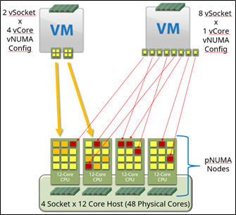
Figure 1: Example Logical CPU Configuration
Figure 1 shows two different VM vCPU configurations, even though both were configured with eight vCPUs. The first VM on the left is configured with two virtual sockets (smaller CPU scheduling footprint per NUMA node), each with four virtual cores. The second VM on the right is configured with the default configuration of eight virtual sockets, each with one virtual core. The first example is configured to equally scale across two physical CPU sockets, which might be optimal given the workload on each CPU socket. The memory access patterns are kept confined to just the two sockets, and the VM knows how to efficiently manage the memory lookups on each vNUMA node. The second example is potentially scattered across all available pCPU sockets and cores, and the memory management is not optimal and results in a performance loss.
Take the example of a SQL Server VM that requires 16 vCPUs to appropriately handle the workload. Which of the following configurations is the right vCPU configuration?
- One virtual socket with 16 virtual cores
- Two virtual sockets, each with eight virtual cores
- Four virtual sockets, each with four virtual cores
- Eight virtual sockets, each with two virtual cores
- Sixteen virtual sockets, each with one virtual core
The answer is the standard DBA answer – “it depends”. It all depends on your underlying hardware, the amount of resource contention occurring on the physical machine, and the NUMA awareness of the application. Fortunately for us, SQL Server is extremely NUMA aware. So, you can configure the VM for a certain configuration, run a workload stress test or a synthetic benchmarking utility (configured to mimic your workload characteristics), and get some performance metrics. For your business critical applications, I would evaluate the performance of multiple vNUMA configurations and determine the configuration that yields the most optimal performance.
Does it really make a difference?
In a nutshell, yes. The above example in Figure 1 was tested on a new VM environment a few months back, and the results will surprise you. A new VM was constructed and tested with three difference vCPU configuration: four vSockets by four vCores each, eight vSockets by two vCores each, and two vSockets by eight vCores each. HammerDB was used to perform a SQL Server workload stress test. The results from the stress test were graphed by number of concurrent users.
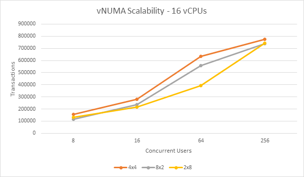
Figure 2- vNUMA Scalability
In this test, the configuration with four virtual CPU sockets, each with four virtual CPU cores, came out on top during each test. At 64 concurrent users, this configuration was 31% faster than the two virtual sockets by eight virtual core configuration.
That’s a dramatic improvement for not having to touch a single line of code. The best part of this improvement is that it’s completely free.
The goal is to configure a VM that is configured with the appropriate number of vCPUs for the workload, with a proper vNUMA configuration that best matches the server CPU architecture underneath. If the memory assigned to the VM spans a NUMA node, split the VM into two or more vNUMA nodes to reduce the cross-node lookups. Make sure that the physical hosts your VM might be able to run on have the same hardware configuration. If different configurations exist, test the performance on all distinct hardware configurations and select the VM configuration that works the best in all scenarios.
Hot-Add
Hypervisors have the ability to hot-add, which is the ability to add CPUs and memory while the VM is powered on. However, let us consider the NUMA implications. If you have four vCPUs and 16GB of RAM on a VM configured with one virtual CPU socket, and then added thirteen virtual CPUs to the VM to bring it to a total of seventeen, how would the NUMA balancing handle it? Technically, it’s possible to accomplish this, but unless the physical host underneath the VM contained CPU sockets with equal or greater numbers of physical CPU cores, it would most likely handle it poorly because of memory lookups that span NUMA boundaries. Therefore, if you have any sort of hot-CPU or hot-memory add feature enabled at the VM layer, vNUMA extensions are not enabled at all. You will most likely take an ongoing SQL Server performance hit because of the memory NUMA lookups underneath the virtual machine if hot-add of CPUs or memory is enabled.
It is recommended to not enable hot-add on a SQL Server VM, which removes vNUMA extensions and possibly hurts performance, unless your specific circumstances dictate doing so.
Virtual Networking
Virtual machines need a way to connect to a network segment on a physical network. The hypervisor accomplishes this is by creating a named virtual network. This network is mapped to a virtual switch, essentially a traffic routing engine inside the hypervisor. The virtual switch is then connected to one or more physical network adapters on the physical host. When a virtual network adapter on a virtual machine is assigned to a particular named virtual network, the traffic routes out to the physical network through these layers.
Multiple virtual networks can be created. Traffic can be segregated or directed in a number of directions, usually through the extension of a VLAN. A VLAN allows traffic to be isolated or routed in a certain manner, all while multiple VLANs can share a physical network adapter port. A virtual network can be assigned a VLAN tag, which assigns that traffic to a particular VLAN.
Describe your networking requirements to your VM administrators and they should be able to configure the networking layer for you.
For example, let’s say you wanted to configure Availability Groups in virtual machines, and you want to isolate Availability Group communication and backup traffic. In this diagram, three virtual networks, represented by the colored lines, are present for use for virtual machine traffic.
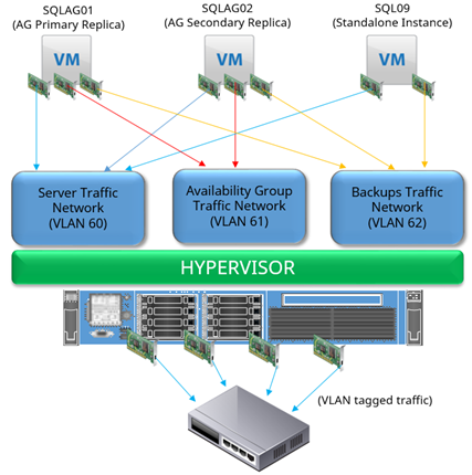
Figure 3- Example of a virtual network
The two SQL Servers that are part of the Availability Group (SQLAG01 and SQLAG02 shown above) contain three virtual network adapters. The third stand-alone instance (SQL09) just contains two. Each of these adapters is connected to an individual virtual network. Each virtual network is configured to use a separate VLAN tag, or VLAN assignment. If the networking underneath is set to not route traffic across VLANs, one server’s network adapter on one VLAN would not be able to “see” the network adapters on other VMs that are not assigned to the same VLAN.
For example, in the above diagram, SQL09 would not be able to access the Availability Group replica traffic taking place on VLAN61.
The flexibility that this presents is limitless. Availability Group traffic can be isolated to allow for the maximum performance without worrying about network congestion from other virtual machines. Backup traffic can be isolated for security purposes. Virtual firewalls can be used to further enhance security, all while eliminating complex physical cabling nightmares or having many network adapters on each physical machine.
Virtual Disks
 Storage can be presented to a virtual machine in a number of ways, all of which have their benefits and drawbacks.
The primary method used by most VM admins is a virtual disk, shown in Figure 4. This would be a VMDK on VMware and a VHDX on Hyper-V. A virtual disk is a file placed on a shared file system managed by the hypervisor (referred to as a datastore), and provides the most flexibility from a hypervisor standpoint. The virtual disk can be relocated dynamically or expanded without disruption to the corresponding guest system. For SQL Server virtual machines, this method is most commonly used.
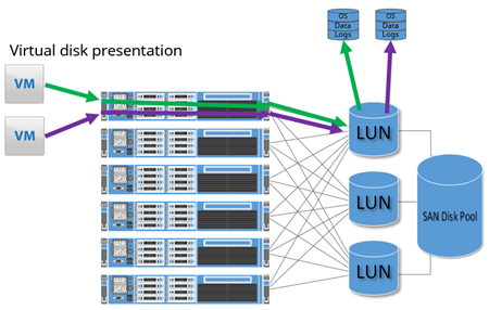
Figure 4- VMDK Illustration
A second method is with a Raw Device Mapped disk (RDM) on VMware, or a Pass-Through disk on Hyper-V. A SAN LUN is carved off and presented to all of the physical servers in the virtualization cluster. In figure 5, this type of disk is represented by the red arrow and box. However, instead of allowing the hypervisor to format and manage it for virtual disks, it is configured to be assigned just to one virtual machine, and is “passed through” the hypervisor and directly connected to the virtual machine. The end result is similar to presenting a single SAN LUN directly to one physical machine.
However, only a couple of reasons exist to justify the use of RDMs/Pass-Through Disks – volume size limitations in VMDKs in older versions of the hypervisors, and VMware-specific shared disk locking for applications like Windows Server Failover Clusters with shared storage. Previous versions of the hypervisors limited a virtual disk in size to 2TB, but vSphere 5.5 expanded this limit to 62TB for both VMDKs and RDMs and Hyper-V expanded to 64TB. In the past, RDMs/Pass-Through Disks outperformed virtual disks but the difference in modern hypervisors is so miniscule that the performance is considered equal.
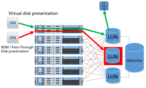
Figure 5- RDM Illustration
A third method of presenting virtual machine disks is with in-guest presentation, usually with iSCSI or SMB 3.0. In-guest presentation allows the VM’s OS itself to be in control of connecting to a storage target, rather than the hypervisor. This method presents the advantage of being able to swing disk targets between a physical machine and a virtual machine by just repointing the LUN from one server to another. This design can be beneficial when migrating large workloads from a physical server to a virtual server with low amounts of downtime. However, this configuration removes the abstraction from a particular device, and therefore reduces the flexibility of the VM when compared to using virtual disks.
Unless an alternative is absolutely required, virtual disks are the preferred method for virtual machine disks presentation.
Before the virtual disks can be presented, profile not only your source SQL Server instance, but also the source server itself. Workloads might exist on that server outside of the scope of SQL Server. Based on this profile, determine the appropriate virtual disk configuration for your workload.
In the example below, eight virtual disks are to be added to a virtual machine based on a specific workload profile, and the drives have been assigned sample sizes.
| Drive | Size (GB) | Purpose |
| C: | 60 | Operating System |
| D: | 20 | SQL Server Instance Home |
| E: | 20 | SQL Server System Databases (master, model, msdb) |
| F: | 100 | User Database Data Files (1 of X) |
| L: | 40 | User Database Log Files (1 of Y) |
| T: | 50 | TempDB Data and Log Files (1 of Z) |
| Y: | 50 | Windows Page File |
| Z: | 100 | Local Database Backup Target |
Note that not all SQL Server workloads need a configuration as spread out as shown in the table above. In environments where SQL Server is only lightly taxed, the configuration could resemble the following.
| Drive | Size (GB) | Purpose |
| C: | 80 | Operating System + SQL Server Instance Home |
| F: | 100 | User Database Data Files (1 of X) |
| L: | 40 | User Database Log Files (1 of Y) |
| T: | 50 | TempDB Data and Log Files (1 of Z) |
| Z: | 100 | Local Database Backup Target |
Just as with a physical SQL Server, the goal is to attempt to split the workloads up as necessary to best distribute the workload across all available queues and paths at each layer of the system stack. If only one worker thread is available for one process, any one of the paths from one end to the other end of the system stack can get congested and become a system bottleneck. This path through the system stack, below in Figure 6, represented by a SQL Server database with one file group (Primary FG) and data file (DF1) residing on one volume (drive E:). The storage request would traverse through one path inside the Windows OS into the virtualization layer, and be sent out one fiber HBA through a single path on the interconnect switches, and finally make its way into one port on the SAN controller and into the disks.
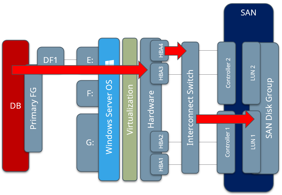
Figure 6– Bottleneck Example
Adding multiple file groups, data files, virtual disks, and ensuring efficient path segregation can minimize the bottleneck possibilities by allowing the hypervisor and physical layers to better distribute this workload. Figure 7 below represents multiple file groups, each with two data files (DF1 through DF4), placed on a few volumes, and therefore the load has the ability to get more efficiently distributed down through the layers to disk.
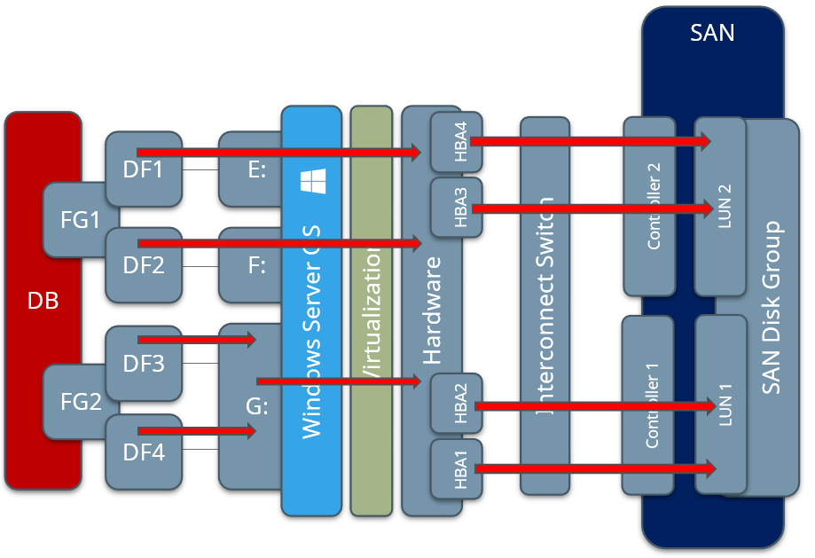
Figure 7– Properly Distributed Workload Example
Separation of workload purposes and types also presents the end user with flexibility in how volumes can be managed. For example, if a Windows or SQL Server Service Pack is about to be applied, the administrator now has the ability to create a VM-level snapshot (point in time rollback point, including the contents of memory) on only the required virtual disks, but might elect to exclude the database volumes so as not to lose already committed transactions if the system state is rolled back.
SQL Server System databases – master, model, and msdb – are split into their own volume because if the system has an implemented feature that has higher utilization, such as mirroring or Availability Groups, this virtual disk can be placed onto a faster tier of storage to provide better performance.
The Windows operating system page file is separated (sometimes, but not always) if heavy SAN-to-SAN replication for DR purposes is in use at an organization. This file placement in the non-standard location allows this individual virtual disk to be placed on a SAN volume that is replicated far less frequently than the others, which saves replication bandwidth.
The database backup target disks are only in use if backups are saved locally and fetched by an external process, instead of using a network location as a backup target. Just as with the Windows system page file, this volume can be placed on slower or less expensive disks to save on costs.
TempDB is broken out onto its own drive because of the nature of the workloads that TempDB handles. If TempDB is subject to large volumes of traffic and you find that you have TempDB contention in the form of storage waits, you can elect to move some of the data files or log file to another virtual disk.
The same methodology goes for the user database and log disks. Your workloads are always different, so weigh the amount of data being actively used on the disks and attempt to balance joined or dissimilar workloads on multiple virtual disks whenever possible.
Summary
Understanding the core configuration options when constructing a virtual machine is necessary before you start the actual VM construction process. Understanding the workload characteristics of your original physical server is important so you can size the virtual machine appropriately. If the machine is already virtualized, check the VM resources and resource configuration to ensure that the VM is “right-sized”. The next two Levels outlines the VMware and Hyper-V-based build processes. Stay tuned!