

Introduction
Forecasting is a very common business process, with which most companies address in a full blown demand planning system. The benefit of such a system is that many different forecast models can be tested for the best fit and applied appropriately through the life cycle of a product. However, it is sometimes necessary to perform forecasting or elements of forecasting outside the demand planning system, generally for ad hoc analysis.
So, if you are ever given the task of creating a time series forecast, with T-SQL as your tool, you will probably start by using one of the most common forecast models: simple linear regression with trend and seasonality. This forecast method is also known as the Holt-Winter’s model and its application will be the subject of this article. One take away is the demonstration of forecasting, though another useful aspect is the illustration of the math to calculate a trend line for a chart.
Simple Linear Regression
Simple linear regression finds the slope (or trend line) within a time series and continues that slope forward to predict a future outcome. The seasonality is then derived from the historical data and applied to the future trend. Seasonality, or periodicity, is a regular fluctuation in demand. For example, the month of December may spike due to holiday sales and August may slump because of the travel season. This could be expressed as a percent variance from the trend line.
Time series forecasts are typically created at a monthly level and broken down to a weekly or daily level, as needed. The monthly breakdown may simply be a function of a weekly mask (% for each week of the month) or it may be a something more complicated as an annual mask. More often than not, it is structured to a fiscal time period. Forecasters prefer the monthly altitude because it is a high enough level for good forecast accuracy while still low enough to detect seasonality and be useful to the business community. For example, think of the challenge in forecasting one item at the ship-to level for each day of the year as compared to forecasting sales for the entire business for the whole year with no ship-to break out. The latter annual forecast will certainly win in overall accuracy.
One last note before getting started, Analysis Services (SSAS) offers a couple of great tools for forecasting that would be infinitely easier to use, if the environment is already built. The first are linear regression functions that are part of Multidimensional Expressions (MDX). These functions pared with others could easily replicate the steps below, in a much simpler way (provided you are comfortable with MDX). However, these functions are broken into pieces to add flexibility in how they are put together, allowing for an additive regression vs. multiplicative, for example. The formulas below should help make clearer the intent of these functions.
The second is the forecasting model that is part of the data mining tools in SSAS. Microsoft uses an algorithm it refers to as Auto Regressive Tree with Cross Prediction (ARTXP), which essentially acts like linear regression, but corrects itself very quickly. By correction I mean that if you were to follow a trend that was steadily growing for 3 years and then suddenly the data started to decline very rapidly, the linear regression trend line will take more than a few periods to start to acknowledge this change and get on the right path again. Often, some sort of moving average like Auto-Regressive Integrated Moving Average (ARIMA) or exponential smoothing will follow this pattern better. The data mining forecast tool uses ARIMA to correct the trend line quickly. Also, ARTXP can use cross correlation (with Enterprise Edition) to detect relationships across products. This could be used to inform the forecast, when an increase in one product might cannibalize the sales of another.
The Forecast Process
This forecast process has three major parts as follows:
1. Prepare the historical data
2. Find the slope and seasonality
3. Create the future forecast and apply seasonality
Step 1 – Prepare the Historical Data
In step one, the historical data is prepared by cleansing it of abnormalities. This is typically done by:
- removing promotional effects,
- smoothing (or de-seasonalizing) the data.
Promotions generally cause a dip before and after the promotional period and inflated sales during the promotion. It is not desirable to have this information in the sales history, because promotions are generally non-repeating events – they will likely not be to the same customer, for the same item during the same time each year for the same amount off with the same ad support, etc.
A wise old forecaster tipped me off one day that the best way to remove promotions is by using a central moving median (this, as opposed to a moving average). A “central” moving median or average uses a certain number of periods before and after a given period. A normal moving average uses the periods before a given period to find the average. The effect is that the average will trail behind an event, no matter the number of periods used. The “median” is simply the middle value in a set of data. A median is a great choice because it cuts across the data where an average will generally show some sign of a spike, however subdued. Figure 1 illustrates the difference – note how the moving average (the red line) rises after the event in week 26, but the median (the green line) cuts straight through.
Figure 1
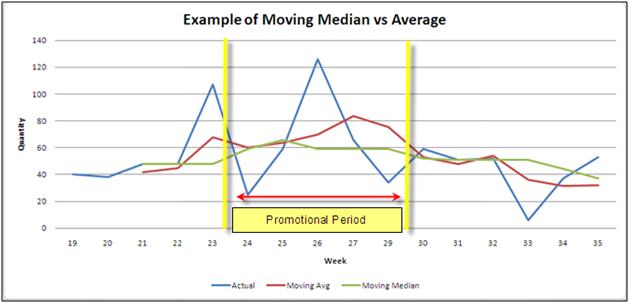
Lastly, the smoothing (or de-seasonalizing) process uses the central moving average. In this case, we wish to retain the seasonal influence but dampen the fluctuations in the data. De-seasonalizing is done so that a better trend line can be extracted from the time series.
In the example (available for download), I start at the point in the process when promotional effects have been removed and the data has been aggregated to a monthly level. I start by creating a table variable to store the results. The table has the following columns:
- Forecastkey (integer, not unique)
- Year (integer)
- Month (integer)
- Product (varchar)
- Baseline Quantity (integer)
- Smoothed Quantity (integer)
- Trend (Numeric(38,17))
- Seasonality (Numeric(38,17))
- Forward Trend (Numeric(38,17))
- Forecast (Numeric(38,17))
The forecastkey is simply a value that increments by 1 for each period record for an item. It starts over for each new item. This column is used for the math in the linear regression – it is very important that the table is ordered by Product, Year, Month, so that the forecastkey has the correct incremental values. Year and month are used, but in a practical application, these would be replaced by a datekey tied to a time dimension.
The baseline quantity is the sales amount stripped of promotions. The smoothed quantity is the baseline amount, smoothed by a central moving average. The trend is the trend line for the historical period. Seasonality is calculated as a ratio of the baseline amount to the trend. The forward trend does not need to be included, but is there to illustrate the creation of a forward trend line. Lastly, the forecast is the forward trend multiplied by the seasonality.
The last four columns have a huge numeric value to avoid rounding errors that could arise during the calculations of these columns. They do not, by any means, imply the level of forecast accuracy. In spite of everything, all forecasts are wrong. Good forecasts are just less wrong.
In the first step, we insert the historical data into the table variable and then update the smoothed_quantity column with a central moving average. We find the average by joining the table to itself on product and forecast key. Remember that the forecastkey is simply and integer that increments by one for each period for a product. In the code snippet below, we join by finding the difference between the keys for a range from -3 to 3. This means that we are looking at 3 periods before and after the period that we are updating and finding the average of all of these periods.
Code snippet:
 Update
       @ForecastTable
 SET
       Smoothed_Quantity = MovAvg.Smoothed_Quantity
 FROM(
       SELECT
             a.ForecastKey as FKey,
             a.Product as Prod,
             Round(AVG(Cast(b.baseline_Quantity as numeric(14,1))),0) Smoothed_Quantity
       FROM
             @ForecastTable a
       INNER JOIN
             @ForecastTable b
       ON
             a.Product = b.Product
            AND  (a.ForecastKey - b.ForecastKey) BETWEEN-3 AND 3
       GROUP BY
             a.ForecastKey,
             a.Product) MovAvg
 WHERE
       Product = MovAvg.Prod
       AND ForecastKey = MovAvg.FKey
The smoothed quantity will help us find a more reliable slope in the data that will be less influenced by outlying data points.
Step 2 – Finding the Slope
In step two, we find the slope and calculate historical seasonality. This is done by solving the equation y = a + bx. This looks a lot like y = mx + b and I really have no idea why the variables are flipped around in this equation, but the former is what is used in text books for linear regression. If you remember back to high school trig, you may recall the terms “rise” and “run” in reference to the slope of a line. In the equation above, the slope (run) is “b” and the y-intercept (or rise) is “a.” A really great resource to explain the rest of the math is http://www.easycalculation.com/statistics/learn-regression.php. The SQL statement below illustrates how this formula can be solved with SQL.
The formulas to solve “a” and “b” are as follows:
- Slope(b) = (Count * SXY - (SX)(SY)) / (Count * SX2 - (SX)2)
- Y-Intercept(a) = (SY - b(SX)) / Count
where S means “the sum of.”
To accomplish this task in SQL, I created a second table variable to complete the calculations and store them by product. By later joining this table variable to the first table variable which holds the data that we will forecast, we avoid using a cursor and looping through one item at a time. This new table variable has the following columns:
- Product (nvarchar(25)) – the product identifier
- Counts (int),
- SumX (Numeric(14,4)),
- SumY (Numeric(14,4)),
- SumXY (Numeric(14,4)),
- SumXsqrd (Numeric(14,4)),
- b (Numeric(38,17)),
- a (Numeric(38,17))
| Column Name | Data Type | Description |
| Product | Varchar(25) | Product identifier |
| Counts | int | The count of all historical rows for an item |
| SumX | Numeric(14,4) | The sum of the forecastkey. You can think of this as a representation for time which would place on the X-axis if we charted it. |
| SumY | Numeric(14,4) | The sum of the smoothed quantity (of the value for our Y-axis). This is the historical value that we are creating the forecast for. |
| SumXY | Numeric(14,4) | The sum of (the forecastkey * the smoothed quantity) |
| SumXsqrd | Numeric(14,4) | The sum of the forecastkey to the power of 2 |
| b | Numeric(38,17) | The Slope (the formula will follow in more detail below) |
| a | Numeric(38,17) | The y-intercept (the formula will follow in more detail below) |
The first column identifies the product – one calculation will be stored for each item and applied across all historical rows. The next 5 columns are used to calculate “b” and “a” from the formula y = a + bx. Later, when we calculate the forecast, “x” will be the forecastkey.
This 2nd step in the forecast process is achieved in three substeps. First, the calculations for Counts through SumXsqrd are solved:
Code Snippet
SELECT
       Product,
       COUNT(*),
       sum(ForecastKey),
       sum(Smoothed_Quantity),
       sum(Smoothed_Quantity * ForecastKey),
       sum(power(ForecastKey,2))
 FROM
       @ForecastTable
 WHERE
       Smoothed_Quantity IS NOT NULL
 GROUP BY
       Product
In the code snippet above, product will be our key for joining to the historical table. The “where” clause is used to ignore rows without a smoothed quantity. This can be useful if the forecast is stored in a permanent table and will be updated each month as actuals arrive into the table. In other words, you would not want to include forecast rows in your calculation.
Next, we calculate “b” using the calculations we just made:
b = ((tb.counts * tb.sumXY)-(tb.sumX * tb.sumY))/(tb.Counts * tb.sumXsqrd - power(tb.sumX,2))
In high school, we calculated a slope between two points. This calculation calculates a slope through an array of points. This is the reason why smoothing of the historical data is so important, because it helps to limit the effect of outliers and improve the accuracy of the slope.
Finally, we calculate “a” with the following:
a = ((tb2.sumY - tb2.b * tb2.sumX) / tb2.Counts)
This calculation finds the point where our slope from above will intersect with the Y-Axis. This is important because it gives reference to the starting point of a forecast – are we selling 10 a month or 10,000? The y-intercept will be used in our forecast calculation to place the total quantity in the right range.
Step 3 – Creating the Future Forecast
In the last step, we create a loop to insert future forecast records by joining the historical data with the calculations table variable. In this exercise, we will forecast 12 periods ahead, so we loop 12 times, each time inserting a row for each product and incrementing the forecastkey by 1. We find the last forecastkey by finding the max(forecastkey) for each product.
The next columns that we insert are the year and month. If this were a dataset that we would add a new forecast row each month, we would want to find the year and month dynamically which could be done by adding a column to carry a date for each first of the month. Then the year would be Year(DateCol) and the month Month(DateCol). Alternatively, if these were fiscal periods, you could find these future periods by joining to a date table.
After we add the month and year (and product) to analyze out data, we calculate the trend (or forecast without seasonality) and we calculate the forecast with seasonality. The trend is not essential to the process, but it is nice to include in charting to more clearly demonstrate the direction of the forecast. To calculate the trend, we return to the formula y = a + bx:
MAX(A)+ (MAX(B)* MAX(Forecastkey)+ 1)
The max() function is only used because we need to fine the last forecastkey for each item, it has no effect on the values for “a” and “b” from our calculation table. To find the forecast, we use the same formula as above and multiply this by the average seasonality for the item:
Code Snippet:
MAX(A)+ (MAX(B)* (MAX(Forecastkey)+ 1))
 *
 (SELECT
       Case WHEN avg(Seasonality)= 0 THEN 1 ELSE avg(Seasonality)END
   FROM
       @ForecastTable SeasonalMask
   WHERE
       SeasonalMask.Product = a.Product
      AND SeasonalMask.CMonth = @Loop +1)
This sub-select statement returns the average for the seasonality column for the particular month that we are forecasting for. The case statement eliminates making the forecast 0 if the average trend turns out to be 0 for some reason. Lastly, we review the results. I suggest playing with the data in excel to see how results came out. Figure 2 shows a snapshot of this.
Figure 2
Summary
This article demonstrates one of the most common forecast models – linear regression, and shows how to apply the forecast formulas in a SQL environment. While users could perform these same formulas in excel, this exercise offers an alternative by creating a database driven forecast. While no forecast model is a one size fits all for every application, linear regression provides a window into forecasting and offers a level of sophistication beyond moving averages. This code could be used for forecasting sales data or even simply used for showing a trend line of data in a chart or for creating ad hoc forecasts.
Edit
2017-04-20
James Waugh noted an error in the order of operations for two lines of this code. Specifically, the element below:
MAX(B) * MAX(Forecastkey) + 1
Should be:
MAX(B) * (MAX(Forecastkey) + 1)
This had a slight impact on the forecasted amount and trendline, causing them to be slightly lower.
Thanks, James!
Mark
