
As we do customarily in the Levels of this series, we'll discuss ways in which BLANK() can be employed, first, in this Level, in "standalone" examples for the function, and then, in Level 5, in situations where we combine it with other functions (specifically the ISBLANK() function), to achieve a result similar to something we might need to generate for clients or employers in our own environments. As part of our exploration of the BLANK() function, we will:
- Discuss the nature of missing or empty values in a DAX expression;
- Examine the syntax involved in using the function;
- Undertake illustrative examples of the uses of the function in practice exercises;
- Briefly discuss the results datasets we obtain in the practice examples.
In addition to introducing the BLANK() function, we will examine the output we obtain via a calculated column we construct within the PowerPivot window in the practice session that follows. We will further create a measure, within a new PivotTable, that puts the BLANK() function to work, to replicate the behavior that we have examined in the calculated column created in the PowerPivot window. As is typically true within the Levels of this series, we will compare and contrast differences in use and behavior of the DAX function under immediate consideration in calculated columns and calculated members in general, and discuss criteria to consider in choosing which of these calculation types to exploit to meet requirements we encounter in supporting employers and clients.
Preparation for the Levels of the Stairway to PowerPivot and DAX Series
As we'll note throughout, to obtain the most benefit from the Levels of the Stairway to PowerPivot and DAX series, you will need to have installed the PowerPivot for Excel 2010 add-on on your machine, or to have installed Excel 2013 and enabled it to work with PowerPivot. You will also need to have installed SQL Server 2008 or above (including Analysis Services) and the respective relational and Analysis Services samples on your local machine, or have the client portions of each on your machine with access to the rest on a server. To perform all Levels of preparation, see the installation section of the charter Level of this series, Level 1: Getting Started with PowerPivot and DAX.
Preparation for the Practice Exercises in this and the Next Levels
Once we';ve got the PowerPivot for Excel 2010 add-in (or Excel 2013), SQL Server 2008 or above, and the samples noted above installed, we're ready to perform the practice exercises within this Level. Importing the sample database and taking other preparatory steps are critical to providing the environment required to successfully complete this Level, and should be performed before beginning.
Because we will work with different data sources throughout this series, the steps of environment preparation will be repeated in various steps. The objective is to make each Level a freestanding session that can be completed independently of other Levels, so that you can focus upon gaining exposure to the specific skills required to meet your own immediate requirements efficiently. Where appropriate, references to functions, procedures and other details will be supplied, but the objective of each Level is to focus upon one or more specific DAX functions and / or PowerPivot / PivotTable procedures to satisfy needs that mirror requirements we encounter in our own business environments.
1. From the Start menu, select Microsoft Excel 2010 (or above).
2. Within a new, blank workbook, above the Excel ribbon, click the PowerPivot tab.
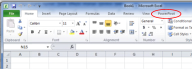
Illustration 1: Click the PowerPivot Tab
The PowerPivot ribbon appears.
3. Click the PowerPivot Window Launch button, appearing at the left of the newly appearing PowerPivot toolbar.
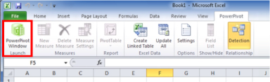
Illustration 2: The PowerPivot Window Launch Button on the PowerPivot Ribbon
The PowerPivot window, containing its own ribbon, opens atop the existing Excel spreadsheet, assuming the name of the workbook as its own name, and defaulting to the PowerPivot Home tab.
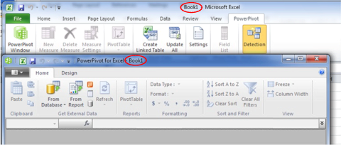
Illustration 3: The PowerPivot Window Associated with the Workbook Appears
Next, we'll designate a source from which to import data.
4. Click the From Database button on the Home tab of the PowerPivot window.
5. Select From SQL Server on the drop-down menu that appears next.
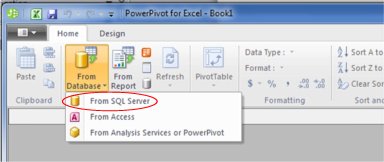
Illustration 4: Select "From SQL Server" in the From Database Dropdown
The Table Import Wizard dialog opens next.
6. In the top input box, titled Friendly connection name, type (or copy and paste) the following:
AdventureWorksDW2008R2
7. Select a server, by either clicking the selector (downward pointing arrow) on the right side of the box titled Server name, or by typing the appropriate server name directly (this will, of course, save the time that the PC takes to browse for server names).
8. Enter the authentication as required for the local environment (ideally selecting Use Windows Authentication).
9. Select AdventureWorksDW2008R2 (or the equivalent in the respective Analysis Services 2008 through 2012 environment in which you are working), using the dropdown selector to the right of the box, titled Database name, at the bottom of the dialog.
The Table Import Wizard dialog, with our input, appears similar to that depicted below.
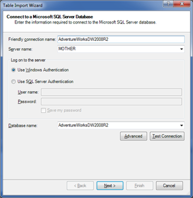
Illustration 5: The Table Import Wizard Dialog, with Our Input
10. Click the Test Connection button underneath the Database name selector.
A message box appears, indicating that the test connection has succeeded.

Illustration 6: "Test Connection Succeeded"
11. Click OK to dismiss the message box.
12. Click the Next button at the bottom of the Table Import Wizard dialog.
13. On the dialog that appears next, labeled Choose How to Import the Data, leave the radio button at its default of Select from a list of tables and views to choose the data to import, as shown.

Illustration 7: Choose "Select from a list of tables" option for Data Import
14. Click the Next button.
PowerPivot loads the tables and views from the selected database into the Select Tables and Views page of the Table Import Wizard that appears next.
15. Select each of the tables listed in Table 1 below by clicking the checkbox to the immediate left of the respective table listing in the Source Table column of the dialog, and changing its name, via the Friendly Name input box, the dialog.
| Table to Select (Source Table) | Change Name to (Friendly Name): |
| DimCustomer | Customer |
| DimDate | Date |
| DimProduct | Product |
| DimProductCategory | Product Category |
| DimProductSubcategory | Product Subcategory |
| FactInternetSales | Internet Sales |
| FactResellerSales | Reseller Sales |
Table 1: "Select Table and Views" Dialog Input
The Select Tables and Views dialog appears, as partially shown, with our selection and related tables checked.
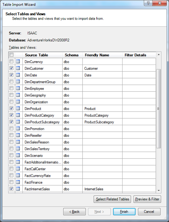
Illustration 8: Selecting Tables (Partial View)
The idea in these immediate steps, once again, is to import enough information into our model to allow us to do some illustrative analysis surrounding the business activities conducted by our hypothetical client, the Adventure Works organization.
16. Click the Finish button.
The import process runs, and then we see a "Success" message, complete with a Details list that indicates population by our choices.
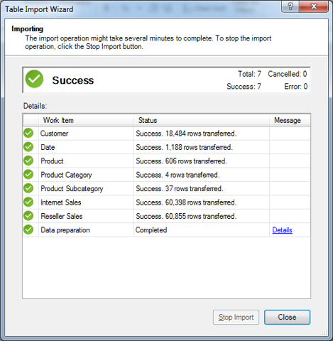
Illustration 9: Success is Indicated, Along with a List of Tables Imported
17. Click Close.
The Table Import Wizard is dismissed, and we arrive at the PowerPivot window once again, where we see the imported data as partially depicted.
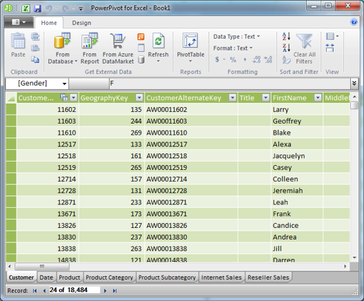
Illustration 10: Imported Data, with a Tab for Each Table
NOTE: For more detailed information about the PowerPivot window itself, please see Level 1: Getting Started with PowerPivot and DAX.
18.Click the PivotTable button atop the current PowerPivot window, as shown.
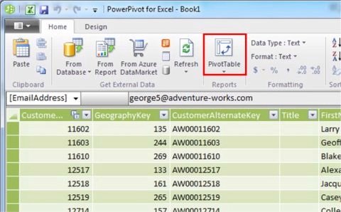
Illustration 11: Click the PivotTable Button atop the PowerPivot Window
We are returned to the Excel worksheet, where the Create PivotTable dialog appears as shown.
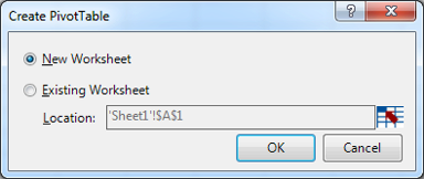
Illustration 12: The Create PivotTable Dialog Appears
19. Leaving the radio button in the default position of New Worksheet, click OK.
20. Click File ? Save As from the main menu atop the worksheet, and save the file to a convenient position as follows:
21.Select Save As from the dropdown menu that appears, as shown in Illustration 11.
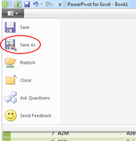
Illustration 13: Select Save As from the Selector within the PowerPivot Window
22.Save the worksheet as ST_DAX04-1.xlsx, placing it in a convenient location.
23.Leave the PowerPivot Window open for the practice session below.
We are ready, at this stage, to get some hands-on exposure to two new DAX functions, BLANK() – in this level - and ISBLANK() – in the next level of our series. Along the way, we will continue to build experience in the general use of PowerPivot to meet business requirements.
Before we dive into these new functions, though, let's take a look at how PowerPivot and Excel handle empty or missing values in general.
Empty Values
As a prelude to our examination of the nature and operation of the DAX BLANK() and ISBLANK() functions, we should gain an understanding of how empty values are treated in
PowerPivot and Excel. The primary reason this becomes important is that empty values often result in calculation errors and / or unexpected results. We must understand how empty or missing values behave in a DAX expression, as well as how we can use the BLANK() function to return an empty cell in a calculated column or in a measure, to effectively control the results of a DAX expression under these conditions.
In SQL Server, as well as within most relational databases, a missing value is treated as "Null." It is typical in relational environments for calculations involving a Null to return a Null by default, although SQL Server and other environments allow for modification of this behavior. In Analysis Services, as well as in other multidimensional databases, missing values are typically treated, depending upon the source data type, as empty strings or zeros.
PowerPivot designates a missing value as a "Blank." When we add a number to a blank value, the number itself is returned, instead of a Null or another blank. In handling missing values, blank values, or even empty cells, DAX uses a value of BLANK. BLANK comprises a way to identify these conditions, and is not a real value itself. To obtain a value of BLANK, which is different from an empty string, we employ the BLANK() function, as we'll describe below.
Excel differs from PowerPivot in its treatment of empty values. Excel interprets an empty value as a zero ("0") when that value is used within a summing or multiplication operation. Moreover, Excel returns an error if empty values are subjected to division, or used within a logical expression.
The BLANK() Function
Introduction
According to the TechNet Library, the DAX BLANK() function "returns a blank." BLANK(), a fundamental and important function, is a member of the Excel Text Functions group.
BLANK() is useful in numerous contexts, and is typically used in conjunction with other functions. A common example of its use, which we'll see in an example later, is a situation where it controls the output of a ratio where, say, the denominator may be empty or a zero. In such a scenario, we might use BLANK() to return a blank value, or empty cell in the PowerPivot window, which it would always do in this expression:
= BLANK()
BLANK(), therefore, offers utility whenever we need to return a blank value, even though the expression above serves no useful end on its own.
We will explore the syntax for the BLANK() function after a brief discussion in the next section. We will then gain some hands-on exposure to its use, within practice examples constructed to support hypothetical business needs. This will allow us to activate what we explore in the Discussion and Syntax sections.
Discussion
To restate our initial explanation of its operation, the BLANK() function returns a blank, plain and simple. To understand how the function can be most useful to us in given business situations, we need to understand how the "empty value" that BLANK() returns can, depending upon the calculation into which it is inserted, return a blank, which, as we'll see, is often the desired outcome.
In DAX, an expression returns a blank in many cases when it contains any "blank" that is operated upon via the expression. This would be true in an instance, for example, where we simply multiplied a constant against a value that was empty, like this:
= FactInternetSales[SalesAmount]*.06
where we are computing a sales tax amount upon an empty or null SalesAmount value in the underlying data. Many (but not all) arithmetic and logical operations generate a blank, in cases where one or both of the "participants" in the operation are blank, it simply depends upon the operation.
Let's look at some syntax illustrations to further clarify the operation of BLANK().
Syntax
To return a blank using BLANK(), we simply supply the function, with nothing in the parentheses to the right of the BLANK keyword, like this:
BLANK()
For example, let's get a feel for the general use of BLANK() within the InternetSales tab of the PowerPivot window, where we have performed the imports described in the Preparation section above. Let's say we want to put BLANK() to use in a scenario where we wish, within a calculated column, to return a blank in any row where we have a Sales Amount of less than $ 500.00, but to return the actual Sales Amount value in any case where the value is equal to or greater than $500.00. A straightforward way to accomplish this would lie within the following formula:
=IF(InternetSales[SalesAmount]< 500, BLANK() , "> $ 500.00" )
If we looked at the new calculated column on the tab, at a point where we have both possible conditions in the SalesAmount column, we would see something like this:
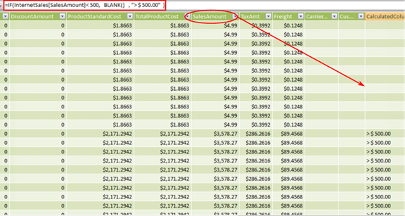
Illustration 14: Calculated Column Using BLANK() on the InternetSales Tab (Partial View)
As is obvious, within the small view we see above, the calculation delivers the required "bucketing:" in rows where Internet Sales are less than $ 500, a blank, or empty, is returned, whereas in those rows where we have Internet Sales greater than or equal to the same value, our string of ">$ 500.00" appears. In this simple example, we witness the action of the BLANK() function: to literally return a blank under desired conditions.
Let's get some hands-on practice with BLANK() in the section that follows:
Practice
To reinforce our understanding of the basics we've covered so far, we will follow our typical pattern of employing the function under examination in this Level within the definition of a couple of calculations: First, we'll work with BLANK() via a calculated column within a tab of the PowerPivot window. Next, we'll put the function to use via a calculated measure within a PivotTable of a worksheet within the associated Excel workbook. We will examine the use of BLANK() in combination with other functions with which we work in other Levels. The intent, as in all the practice sessions of the Stairway to PowerPivot and DAX series, is to demonstrate the operation of each of the functions we examine in a straightforward, memorable manner.
Let's move to the Excel worksheet we prepared earlier as a platform from which to construct and execute the DAX we examine, and to view the results we obtain.
PowerPivot Calculated Column
Let's take a relatively understandable business need: We wish to determine the percent discount (when a discount is taken) in each Reseller Sales transaction experienced in the Adventure Works sample. The math is simple: divide the Discount Amount for each row (transaction) in the Reseller Sales table by the respective Reseller Sales Amount. But, because discounts in the table are sparse, we wish to build further logic into the calculation to handle "zero" Discount Amounts within our percentage calculations in such a manner that a blank – not a zero – is returned. (The "blank" presentation is driven by a desire to distinguish "zero percent" from "no discount taken – a minor, but not uncommonly chosen, visual effect.)
We will deliver the desired result with a calculation whose components include the DAX BLANK() function.
2. Return to the PowerPivot Window.
3. Click the Reseller Sales tab.
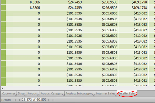
Illustration 15: Click the Reseller Sales Tab
4. Scroll to the right, and then click the top row in the column labeled "Add Column," which appears on the far right side of the tab, as shown.
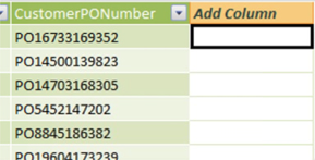
Illustration 16: Click the Top Row in the Column Labeled "Add Column"
5. Select the function button ("fx") to the left of the formula bar next.
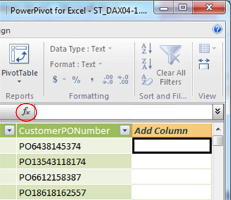
Illustration 17: Select the Function (fx) Button
The Insert Function dialog appears.
6. Click the downward pointing arrow on the selector appearing atop the dialog under the Select a category label.
The following DAX function categories appear:
All
Date & Time
Math & Trig
Statistical
Text
Logical
Filter
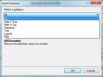
Illustration 18: Insert Function Dialog with Expanded Category Selector
7. Select the Logical category.
8. In the Select a function list that populates for the Logical category, select the IF() function, as shown.
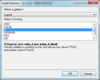
Illustration 19: Select the IF() Function
9. Click OK to confirm the selection and dismiss the Insert Function dialog.
The IF keyword, proceeded by the "=" operator and followed by a left parenthesis ( "(" ), appears in the formula bar, with a function usage tooltip appearing just underneath the function.
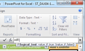
Illustration 20: The Beginning of the IF() Function, along with Tooltip, Appears
10. Because we know that we need now to add the appropriate table name / expression, begin to type in "Reseller Sales."
As we begin to type the table name, AutoComplete immediately presents us with a list of functions and tables from which to select, as shown.
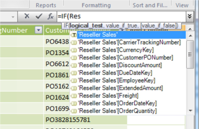
Illustration 21: Table as Suggested by AutoComplete
11. Double-click 'Reseller Sales'[DiscountAmount] within the dropdown list to select the column, as depicted in Illustration 20.
![Select the 'Reseller Sales'[DiscountAmount] Column](/wp-content/uploads/legacy/7f0ef5ba732aea977102ff53f6b3293a461f9d32/17920.png)
Illustration 22: Select the 'Reseller Sales'[DiscountAmount] Column
12. Once the selector is dismissed, and =IF('Reseller Sales'[DiscountAmount] appears in the formula bar, type in the following syntax to the right:
=0, BLANK(),
The syntax to this point should be as shown here:
=IF( 'Reseller Sales'[DiscountAmount]= 0 , BLANK(),
At this stage, the calculation is saying "if the Discount Amount is zero (the logical test), return a blank (the ‘value if true')." We now need to provide the corresponding ‘value if false.'
13. Type the following syntax to the right of the existing expression:
'Reseller Sales'[DiscountAmount]/'Reseller Sales'[SalesAmount])
A completed formula appears within the formula bar.
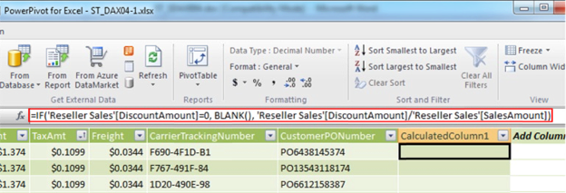
Illustration 23: The Completed Formula Appears
14. Press the Enter key.
The column updates and the formula results appear in each row of the new calculated column, as partially shown below. (Because discounts are sparse in the Reseller Sales table – and zeros exist in most of the Discount Amount rows – the below view is scrolled to capture some sample populated fields in the calculated column.)

Illustration 24: The Results Appear in Each Row of the New Column (Partial, Compressed View)
We note that the value shown in the populated rows appears to be correct. (We would likely format the value, to indicate its "percentage" nature, at the PivotTable report level, as various reporting / analysis needs with regard to decimalization, etc., might differ among presentations.) Let's name the column in accordance with its ultimate intended purpose, at this juncture.
15. Right-click the new column header label (currently at its default of "CalculatedColumn1"), and select Rename Column from the cascading menu that appears.
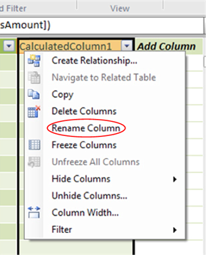
Illustration 25: Renaming the Column to its Ultimate Name
16. Name the newly added column "Disc Perc of Sales" for Discount Percent of Sales.
In the section that follows, we will access the PowerPivot calculated column we have created within a PivotTable. Moreover, we will get some hands-on exposure to putting the DAX BLANK() function to work within a calculated measure we will create in the PivotTable.
PivotTable Measure
In its most fundamental and common use, as we have noted throughout the Stairway to PowerPivot and DAX series, PowerPivot exists to act as a data source for PivotTables. In this section, we will work further with the DAX function we have exposed in the PowerPivot calculated column section above, except this time, we will present calculations and values within a PivotTable.
We can begin our work with a PivotTable from either the Excel workbook or from the PowerPivot window. Because we're already in the latter, we will proceed from there by taking the following steps:
1. From the Reseller Sales tab in the PowerPivot window, click the downward pointing arrow on the PivotTable button to cause the drop-down menu to appear, as shown.
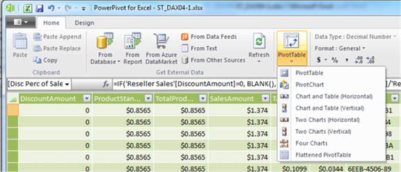
Illustration 26: The PowerPivot Drop-down Menu Appears
While we will work with examples, at various times throughout our series, of some of the other options we see in the dropdown menu (single PivotChart, Chart & Table, Two Charts, Four Charts, and Flattened PivotTable), we will build a single PivotTable in this session, and throughout most of the practice sessions, of our series. This will be the most straightforward (and rapid) avenue to getting hands-on exposure to the underlying PowerPivot data and DAX.
2. Click PivotTable in the dropdown menu we've exposed (the top selection).
We are returned to the Excel window, where we encounter the Create PivotTable dialog, once again.
3. Ensure that the radio button labeled New Worksheet is selected.
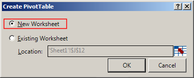
Illustration 27: Ensure the New Worksheet Option is Selected
4. Click OK to accept the setting and dismiss the dialog.
The PivotTable placeholder / canvas, together with the PowerPivot Field List, appear on the new worksheet as depicted (compressed view).
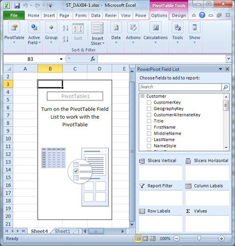
Illustration 28: The PivotTable Canvas Appears on the New Worksheet (Compressed View)
NOTE: Because we cover the details for the first time in an earlier Level of the series, and particularly for those not already familiar with standard Excel PivotTables, Table 1 of Level 2: The DAX COUNTROWS() and FILTER() Functions and More About Calculated Columns and Measures gives a description for each of the areas / zones on the PowerPivot Field List. Other PivotTable basics are discussed there as well.
To gain some exposure to the use of the DAX BLANK() function within the PivotTable, we will replicate some of the steps we took with regard to the Reseller Sales table, upon which we operated in the PowerPivot window in the earlier part of this Level. In accomplishing this, we'll see how to approach what we did with the calculated column earlier, but this time we'll do so with a calculated measure in the PivotTable. Moreover, we will touch upon more PivotTable – specific considerations as we encounter them. But first, we will pull the calculation we created earlier into a new PivotTable we construct, to allow us to compare the results of the calculated column to the calculated measure we create here.
5. Expand the Reseller Sales table in the PowerPivot Field List by clicking the "+" sign to its immediate left.
The columns of the table, with which we worked in the PowerPivot window in the section above, appear.
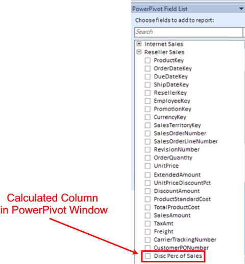
Illustration 29: Reseller Sales Table in the PowerPivot Window, Expanded to Show Fields
The last field in the expanded list, of course, represents the calculated column that we created, and within which we employed the DAX BLANK() function, in the PowerPivot window earlier. We will pull this calculation into our new PivotTable like any other field at this point.
6. Within the PivotTable Field List, inside the expanded Reseller Sales table, scroll to the SalesOrderNumber and SalesOrderLineNumber columns.
7. Drag SalesOrderNumber to the Row Labels drop zone.
8. Drag SalesOrderLineNumber to the Row Labels drop zone, placing it underneath SalesOrderNumber.
The Row Labels drop zone appears, with our two additions, as shown.
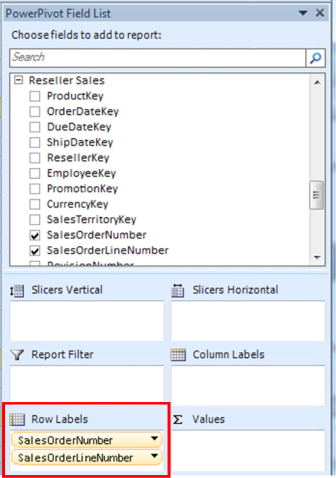
Illustration 30: Creating the Rows Axis of a New PivotTable
9. Again within the Reseller Sales table, click the checkbox to the immediate left of the following columns:
DiscountAmount
SalesAmount
Disc Perc of Sales
The Disc Perc of Sales calculation appears at the bottom of the column listings for the table, and, of course, represents the calculated column we added in the PowerPivot Window earlier. Checking the columns above places each in the Values drop zone (in the order in which we check them) of the PivotTable Field List, where it appears with "Sum of" preceding its name, as shown.
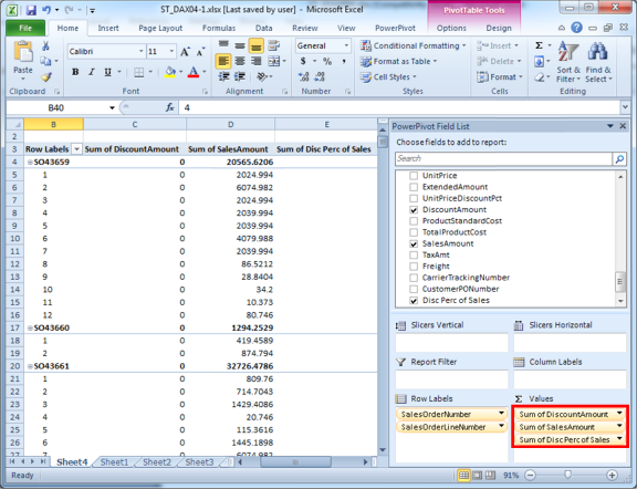
Illustration 31: Adding the Calculated Column to the PivotTable
Because the new PivotTable contains many rows, we will "slim it down" a little for easy review. To do so, we will select just a few Sales Orders to include in the PivotTable.
10. In the upper left corner of the PivotTable, click the cell just underneath the Row Labels selector (the cell containing Sales Order SO43659) to set the context of the dropdown selector, as depicted.

Illustration 32: Select the Top Left Work Order Cell
11. Click the downward pointing arrow of the Row Labels selector, just above the selected cell.
12. Deselect the (Select All) box by clicking the checkmark currently in place, as shown.
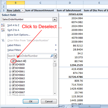
Illustration 33: Deselecting by Removing the Check in the (Select All) Box
Next, let's select a small, contiguous set of Sales Orders to limit the size of the PivotTable with which we will be working.
13. Within the selector, scroll to, and click the check boxes to the immediate left of, each of Sales Orders number SO69401, SO69402, SO69403, and SO69404.
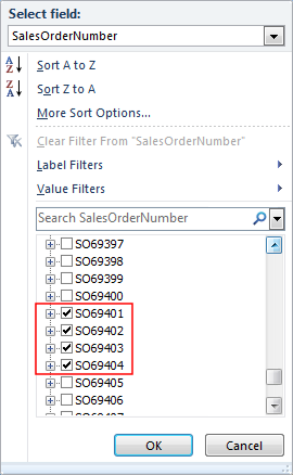
Illustration 34: Select Sales Orders SO69401, SO69402, SO69403, and SO69404
14. Click OK to apply the filter and to dismiss the selector.
Let's focus our attention on the calculated column from the PowerPivot Window that we have added to the (dramatically smaller) PivotTable that now appears. Beginning with the top Sales Order, SO69401, we see that, on the individual lines of the Sales Order, the math appears to work correctly, as well as the logic we';ve enforced to return blank values in cases where the DiscountAmount is zero. For example, on Sales Order Line Number 10, we see that the Disc Perc of Sales calculation delivers 0.052631579, which agrees with the calculation of DiscountAmount / SalesAmount, or 3.9556 / 75.1564.
An issue arises when we test the calculation at the rolled up Sales Order level. In this case, on the total line for Sales Order SO69401, the Disc Perc of Sales calculation delivers 0.251342626, which is incorrect: the Discount Percent of Sales should actually approximate 0.004965131, which differs from what we see in the total line for the Disc Perc of Sales (.251342626).
As we saw in working with the same calculation within the PowerPivot Window in the earlier section, the correct value was being computed at the row level (see Illustrations 23 and 24). It is important to note, as we have pointed out in other Levels of this series, that, when the value is aggregated in the PivotTable, the result is not correct in many cases due to the operation of the SUM() function, which is employed by default when we place a numeric column into the Value drop zone of a PivotTable, among other context-related considerations.
To illustrate further this concept, let's set out to create a calculated measure in the PivotTable that correctly calculates the Disc Perc of Sales value at Sales Order Line and Sales Order levels.
15. Within the PowerPivot Field List, once again, right-click the Reseller Sales table label.
16. Select Add New Measure… from the context menu that appears, as shown.
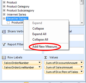
Illustration 35: Select "Add New Measure …"
The Measure Settings dialog appears.
17. Type (or copy and paste) the following into the Measure Name (while leaving the default copied label in place within the Custom Name) box of the dialog.
Disc Perc Total Sales
NOTE: Here we are giving a name that is different from the name we gave the corresponding calculated column in the PowerPivot Window in the section above, simply to make it easy to distinguish the two calculations when they appear within the same PivotTable.
18. Click the function button ("fx") to the right of the Formula label, above the Formula input box of the dialog.
The Insert Function dialog appears.
19. Click the downward pointing arrow on the selector appearing atop the dialog under the Select a category label.
20. Select the Logical category within the expanded category selector atop the Insert Function dialog, just as we did in the earlier exercise.
21. Select the IF() function, once again, as depicted.
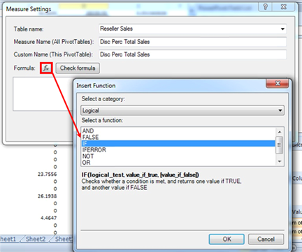
Illustration 36: Select the IF() Function
22. Click OK to confirm the selection and dismiss the Insert Function dialog.
The IF keyword, proceeded by the "=" operator and followed by a left parenthesis, once again, appears in the Formula input box of the Measure Settings dialog.
23. To the immediate right of the left parenthesis (that appears to the right of the IF keyword), begin to type in Reseller Sales.
As we begin to type the table name, AutoComplete again presents us with a list of functions and tables from which to select:
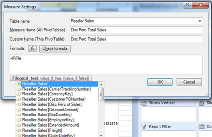
Illustration 37: Functions / Tables as Suggested by AutoComplete
24. Double-click ‘Reseller Sales'[DiscountAmount], as we similarly did at the PowerPivot level earlier, to ensure its selection.
25. Once the selector is dismissed, and =IF('Reseller Sales'[DiscountAmount] type the following syntax to the right, as we did for the similar calculated column in the PowerPivot window in the earlier section of this Level:
=0, BLANK(),
The formula string appears in the formula input box, at this stage, as shown.
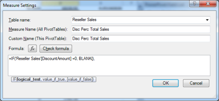
Illustration 38: The Formula Input Box with Formula at this Stage<
As we noted, at this point in creating the corresponding calculated column in the earlier section, our calculation is stating that, if the logical test ("Discount Amount is zero") is true, return a blank. Next, we need to add the value to return if the logical test is false.
26. Type the following syntax to the right of the existing expression within the formula input box of the Measure Settings dialog:
'Reseller Sales'[DiscountAmount]/'Reseller Sales'[SalesAmount])
The completed formula string appears, within the formula input box, as depicted.
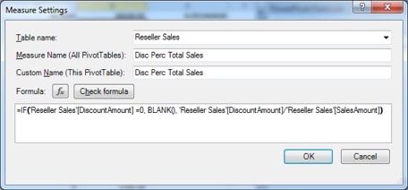
Illustration 39: The Complete Text in the Formula Input Box
The formula string replicates the string we used in creating the Disc Perc of Sales (for Discount Percent of Sales) calculated column in the PowerPivot window earlier.
27. Click the Check formula button.
An error message is returned.
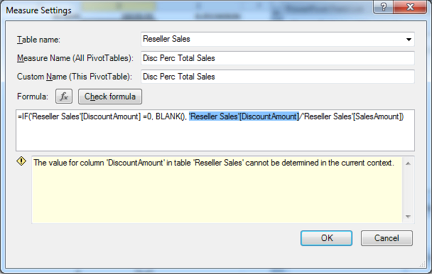
Illustration 40: An Error Regarding Context is Returned
The message indicates that "the value for column 'DiscountAmount' in table 'Reseller Sales' cannot be determined in the current context." It becomes apparent, then, that a calculation that works at the row level, as we saw in our earlier example within the calculated column of the PowerPivot window, fails to generate the correct values in the PivotTable.
What we need, in fact, to do is to pay attention to context, a concept I discuss throughout the Levels of the Stairway to PowerPivot and DAX series. The idea, of course, is to perform the calculation, via our new measure, at the cell level of the new PivotTable and not at the row level of the PowerPivot window. In this case, we must generate the desired value by calculating a ratio that divides the total of 'Reseller Sales'[DiscountAmount] by the total of 'Reseller Sales'[SalesAmount].
Having attempted to use the same DAX expression we employed earlier, only to have received the context error as noted, let's go back and make a couple of minor modifications to our new measure.
28. Modify the syntax currently within the formula input box of the Measure Settings dialog, to place each occurrence of 'Reseller Sales'[DiscountAmount] and 'Reseller Sales'[SalesAmount] within the SUM() function. In other words, modify the existing syntax within the input box from this:
=IF('Reseller Sales'[DiscountAmount] =0, BLANK(), 'Reseller Sales'[DiscountAmount] / 'Reseller Sales'[SalesAmount])
… to this:
=IF(SUM('Reseller Sales'[DiscountAmount]) =0, BLANK(), SUM('Reseller Sales'[DiscountAmount])/SUM('Reseller Sales'[SalesAmount]))
The completed formula string appears, within the formula input box, as depicted.
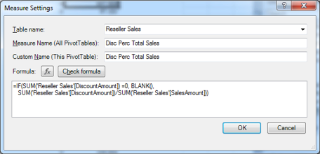
Illustration 41: The Complete, Modified Text in the Formula Input Box
29. Click the Check formula button, once again.
The message returned this time indicates "no errors in formula," as shown.
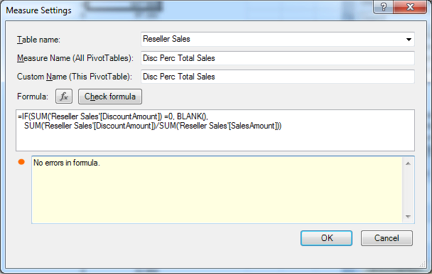
Illustration 42: "No Errors in Formula" is Indicated
30. Click the OK button to accept our changes, and to dismiss the Measure Settings dialog.
The dialog box disappears, and the newly calculated measure appears in a column on the right side of the PivotTable. Let's take a look at the data to ascertain that the values generated by the new measure are correct.
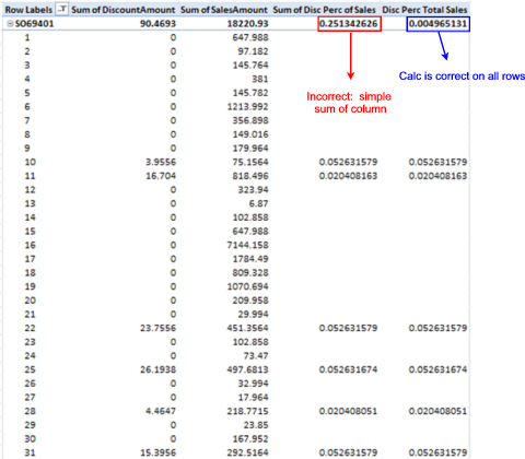
Illustration 43: The New Measure Proves to Be Correct
It's easy to see that, while both calculations appear to return the correct percentage values row-by-row in the individual lines of the sales order selected above, the first calculation (generated when we pulled it into the corresponding calculated column from the PowerPivot window into the PivotTable, by dropping the calculated column from the PivotTable field list into the Value drop zone) simply sums the line item calculations and generates a percentage at the sales order level that is incorrect.
In summary, then, it becomes evident that the value of a calculated column, which is evaluated during data refresh, uses the current row as a context. A PivotTable measure, by contrast, operates upon aggregations of data as defined by the context of the current cell. Source tables are filtered based upon the cell's coordinates, and data is aggregated and calculated via this filter. Put another way, there is no way to reference a single row in a given measure's DAX expression because a measure always operates upon aggregations of data subject to the evaluation (or "filter") context.
We will gain further exposure to the BLANK() function when we use it in tandem with the ISBLANK() function in the level that follows next in our series.
1. From the main menu of the workbook, select File -- Save As …
2. Name the file ST_DAX04-1.xlsx, and save it in a meaningful location.
3. Exit Excel 2010 as desired.
As I emphasize in other Levels, understanding the nature and operation of, the differences between, and the optimal uses for, calculated columns and calculated measures is critical to sound and efficient reporting and analysis when working with PowerPivot. We work with these concepts throughout the Levels of Stairway to PowerPivot and DAX, embellishing and enhancing our technique as the series evolves. Practice and further experimentation with these and other components will ensure that we become fluent in the many options and opportunities that PowerPivot offers the knowledgeable user.
Summary
In this Level of the Stairway to PowerPivot and DAX series, we exposed the DAX BLANK() function. We discussed the general purposes and operation of BLANK(), and then focused upon using BLANK() in general, as well as illustrating ways to leverage the combination of BLANK() and other functions to deliver approaches to meeting business needs. As part of our discussion, we examined the syntax surrounding BLANK(), undertaking illustrative examples of the uses of the function in practice exercises, and then exploring the results datasets we obtained in the practice examples.
We worked with the combination of BLANK() and other functions to deliver illustrative answers to business questions, within both a PowerPivot calculated column and a PivotTable calculated measure we built in the section that followed. Once we had replicated, in the PivotTable, the calculated column we had created earlier in the PowerPivot window, we compared and contrasted the values returned by each, explaining the reasons behind their differences, and discussing considerations in choosing which of these two calculation approaches to take in meeting business requirements in our own environments.