
DAX, which stands for Data Analysis Expressions, comprises the PowerPivot formula language that supports custom calculations in PowerPivot tables and Excel PivotTables. While many of the functions used in Excel are included within the language, DAX also offers additional functions for carrying out dynamic aggregation and other operations with your data. DAX was introduced with PowerPivot, a free add-in for Excel 2010 that promises true “BI for the masses.” PowerPivot holds much promise for analysts, reporting specialists and other information consumers, particularly those who are “at home” with Excel, and who serve the enterprise outside traditional IT and development roles.
PowerPivot offers those who adopt it the capability of creating BI solutions rapidly, and often without the need for the resources required to construct traditional BI solutions. Moreover, my experience has shown that, even in environments where traditional solutions (including everything from ETL mechanisms, underlying star-schema data sources, Analysis Services cubes, and the languages required to support all these components) are desired, PowerPivot can be used effectively to make the design, development and testing of the ultimate solution more efficient and reliable.
The PowerPivot / DAX combination insulates Excel users from many of the complexities of other components of the integrated Microsoft BI solution. The DAX functions are intuitive, in large part, for those that work routinely with existing Excel functions, and enable knowledgeable users to rapidly extract and present the information needed to support enterprise decision makers in a timely, reliable manner. In working with columns and tables (even very large ones) in relational data sources, we can enjoy high-speed lookups and calculations via an in-memory engine that DAX is designed to leverage in an optimal manner
In this series, our primary objective is to become comfortable with creating useful queries, within a business context, using the PowerPivot / DAX combination. As a means of achieving our objective, we will gain hands-on exposure to using PowerPivot in general, while becoming familiar with the DAX language, using formulas we construct from the DAX functions we introduce within the levels of this Stairways series. For each function we introduce, we will discuss what it is designed to produce and its operation in doing so, the syntax with which it is employed, and the data that it retrieves and presents. The objective will be to encourage you to take the example code as you read the ‘steps’, and try it out, making changes and experimenting, so as to get the feel for the capabilities of PowerPivot and DAX. We’ll illustrate every point with practice examples of business needs that we address with practical syntax. Try them out.
To get the most out of the series, you need to have installed either 64- or 32-bit Excel 2010, matched with the respective version of PowerPivot for Excel 2010. PowerPivot for Excel 2010 is, at this writing, a free add-in that is available for download at www.powerpivot.com. For the lion’s share of our practice exercises, which focus upon the Microsoft BI stack, we will use the Adventure Works relational OLTP and Data Warehouse database samples, as well as the Adventure Works Analysis Services database (and the Adventure Works cube it contains) sample, the installation of which we discuss in the section below.
You will also need the appropriate access rights to the sample data sources provided for SQL Server 2008R2. Installation of the Standard edition of SQL Server 2008R2 will be adequate for the vast majority of our activities, although the Developer / Enterprise edition is certainly ideal. I will provide references for step-by-step installation of SQL Server 2008R2 Developer / Enterprise in the section that follows, and the vast majority of the images presented in this series will reflect those environments.
It is also assumed that the computer(s) involved meet the system requirements, including hardware and operating systems, of the applications I have mentioned.
Important Note: If you have no alternative except to work with SQL Server 2005 or 2008, the practice exercises of this series can perhaps be meaningfully completed with modification of the queries to compensate for differences in the data structures of the sample cube among the versions – although you may find this requirement cumbersome and distracting. Because both the relational databases and the Analysis Services samples for 2008R2 differ somewhat from those of previous releases (a good example of this is that the Analysis Services date dimension, as well as the supporting relational data, has been advanced into later operating years of the Adventure Works organization), the sample formula syntax that we construct together will, when executed, deliver results which may differ between 2008R2 data sources and those of the previous releases. While you can adjust your own steps to make up for these differences (perhaps by “checking your answers” independently), you will not have the added comfort of the “instant corroboration” available in simply comparing your results to those presented in the images and explanations I present in the exercises.
Consider working, therefore, with 2008R2, if at all possible: learning the basics of a new language is typically challenging enough for most that are new to it, without the additional distractions imposed by working with older releases.
Additional Note: The screen captures in this series, unless otherwise noted, are made from a Windows 7 or Windows Server 2008 R2 environment, so what you see on your own machine may differ, somewhat, if you are working within another environment.
Installing PowerPivot, Analysis Services 2008R2 and Samples
To install PowerPivot, simply perform the steps as outlined at the download site (www.powerpivot.com, at this writing), on a PC with Excel 2010 installed.
SQL Server 2008 and 2008R2 each provide a virtually identical single Setup program from which you can install any or all of its components, including Analysis Services. Using the unified Setup, you can install Analysis Services with or without other SQL Server components on a single computer. It is important, however, to understand that Analysis Services relies upon other components of SQL Server: for example, the Adventure Works cube (which resides within the Adventure Works DW 2008R2 Analysis Services database), uses the AdventureWorksDW2008R2 relational data mart in SQL Server as its data source, so, if we want to process the Analysis Services database and its cube (we cannot query an unprocessed cube), we will need to have access to its underlying relational data source and, therefore, to SQL Server and the associated sample database.
There are many possible considerations in the installation of Analysis Services, depending upon the version(s) you intend to install, the hardware in your local environment, applications you may already have in place, and so forth. Rather than trying to reproduce them all in this article, we provide the following link, which covers this subject thoroughly, yet efficiently.
Considerations for Installing Analysis Services
(http://technet.microsoft.com/en-us/library/ms143708.aspx)
Once you have determined the components you need to install, you can follow step-by-step instructions on how to start Setup, and to select the components you want to install, by following this link:
Quick-Start Installation of SQL Server 2008
(http://technet.microsoft.com/en-us/library/bb500433.aspx)
Once you have successfully installed Analysis Services (along with any other components you have chosen from the Setup program), you are ready to download and install the samples that we will be working with in this series. A great summary of the options that are available (based upon your SQL Server version and other considerations) can be found at:
How to install Adventure Works SQL DW and Analysis Services 2005/2008 sample database and project
http://www.ssas-info.com/analysis-services-faq/29-mgmt/242-how-install-adventure-works-dw-database-analysis-services-2005-sample-database
Getting Started with PowerPivot
Once we’ve got the PowerPivot for Excel 2010 add-in, SQL Server 2008R2 and the samples noted above installed, we’re ready to get started with PowerPivot. Opening PowerPivot by taking the steps below will put us in position to begin working with DAX formulas. An open PowerPivot window, the point at which we will be at the end of this section, will become the beginning point of each of the levels of this series.
- From the Start menu, select Microsoft Excel 2010.
- Above the Excel ribbon, click the PowerPivot tab, as shown.
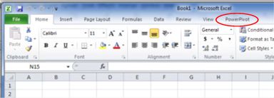
Illustration 1: Click the PowerPivot Tab …
The PowerPivot ribbon appears.
- Click the PowerPivot Window button, appearing at the left of the newly appearing PowerPivot toolbar, as shown.
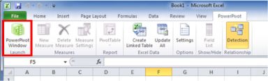
Illustration 2: The PowerPivot Ribbon Appears
The PowerPivot window, containing its own ribbon, opens atop the existing Excel spreadsheet. We can tell to which workbook the window is linked because it assumes the name of the workbook as part of its own name, as depicted below.
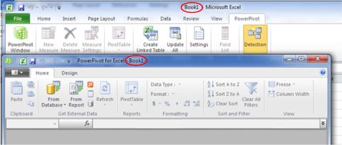
Illustration 3: The PowerPivot Window, Associated with the Workbook, Appears
It is in the PowerPivot window that we load and prepare the data with which we will be working (or will continue working, with data already added to the workbook). We will typically build a relational model here. As we’ll see shortly, the PowerPivot window displays the tables on individual, tabbed sheets, and is the central place where we import tables, create relationships, maintain column data types and formats, and view, as needed, the data that underlies our data model.
Next, we’ll designate a source from which to import data.
- Click the From Database button on the PowerPivot window.
- Select From SQL Server on the drop-down menu that appears next.
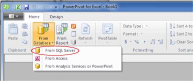
Illustration 4: Select “From SQL Server” in the From Database Dropdown
The Table Import Wizard dialog opens next.
- In the top input box, titled Friendly connection name, type (or copy and paste) the following:
AdventureWorksDW2008R2
- Click the selector (downward pointing arrow) on the right side of the box titled Server name.
PowerPivot begins a scan of the machine to detect, and return to the selector, the available server choices.
- Select the appropriate server for your local environment, or type in the server name / localhost, as appropriate.
- Enter the authentication as required for the local environment (ideally selecting Use Windows Authentication).
- Select AdventureWorksDW2008R2 using the dropdown selector to the right of the box titled, Database name, at the bottom of the dialog.
The Table Import Wizard dialog, with our input, appears similar to that depicted below.
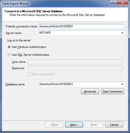
Illustration 5: The Table Import Wizard Dialog, with Our Input
- Click the Test Connection button underneath the Database name selector.
A message box appears, indicating that the test connection has succeeded.
Illustration 6: “Test Connection Succeeded”
- Click OK to dismiss the message box.
- Click the Next button at the bottom of the Table Import Wizard dialog.
- Leave the radio button on the dialog that appears next, labeled Choose How to Import the Data, at its default of Select from a list of tables and views to choose the data to import, as shown.
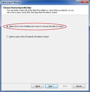
Illustration 7: Choose “Select from a list of tables…” Option for Data Import
- Click the Next button.
PowerPivot loads the tables and views from the AdventureWorksDW2008R2 database into the Select Tables and Views dialog that appears next.
- Select the following tables, by clicking the checkbox to the immediate left of the respective table listing in the dialog:
- DimAccount
- DimCurrency
- DimCustomer
- DimDate
- DimGeography
- DimProduct
- DimPromotion
- DimSalesReason
- DimSalesTerritory
- FactInternetSales
- FactInternetSalesReason
- Click the Select Related Tables button next.
The Select Tables and Views dialog appears, as partially shown, with our selection and related tables checked.
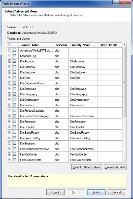
Illustration 8: Selecting Tables (Partial View) …
The idea in these immediate steps is to import enough information into our model to allow us to do some illustrative analysis surrounding the business activities conducted by our hypothetical client, the Adventure Works organization.
- Click the Finish button.
The import process runs, and then we see a “Success” message, complete with a Details pane that indicates population by our choices.
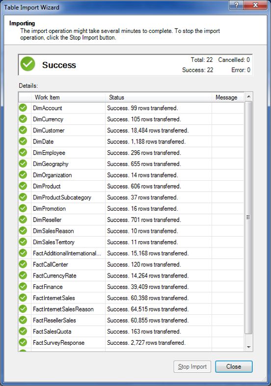
Illustration 9: Success is Indicated, Along with a List of Tables Imported
- Click Close.
The Table Import Wizard is dismissed, and we arrive at the PowerPivot window once again, where we see the imported data as partially depicted.
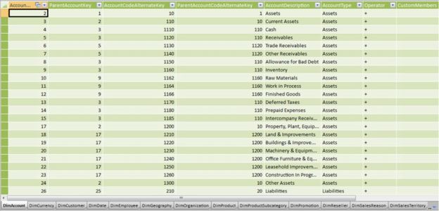
Illustration 10: Imported Data, with a Tab for Each Table
Note that a tab for each imported table has been created in the PowerPivot window (the tabs appear in the bottom left of the window as seen above). What we are now seeing is not an Excel table, but a view of the efficiently compressed columnar database that PowerPivot uses to store imported tables in memory.
The central pane contains the data and looks very similar to – but is not - an Excel table inside a worksheet. Keep in mind that PowerPivot tables and Excel tables are completely different objects: PowerPivot uses far less memory than the Excel tables with which we have become familiar, due to its superior data compression capability. The database generated by PowerPivot saves space and supports highly efficient querying.
Getting Started with DAX
We learned within the introduction to this level that PowerPivot for Excel 2010 offers the DAX language as a means for extending our capabilities with PowerPivot. Let’s get some hands-on exposure to some basic DAX expressions as a way of getting up to speed and positioning ourselves to learn about individual functions in the levels of this series.
We’ll get started with some simple exercises. To begin, let’s assume that we have a need to create a combined Product code / name label, primarily for report parameter picklist support and report labeling, but perhaps for other uses, as well, over time. (We will use the ProductAlternateKey for this purpose, as the ProductKey in the table is a surrogate key, and not the actual product identifier.) This simple concatenation will serve as a great starting point in our introduction to DAX formulas and expressions.
- Click the tab named DimProduct in the PowerPivot window.
- Scroll over to, and click, the header of the far right column on the tab, which is labeled Add Column.
The Formula bar (fx) is activated, upon selection of the column.
- Type (or copy and paste) the following into the Formula bar:
= [ProductAlternateKey] & " - " & [EnglishProductName]
NOTE: We can also use the AutoComplete feature to save typing and / or avoid typographical or syntax errors.
We can use simple column names in the above syntax because the columns reside in the same table as our calculated column. (We have to affix the table name if the column resides elsewhere, as we’ll see in later exercises.)
- Press the ENTER key.
The affected area of the DimProduct tab of the PowerPivot window appears, with our new addition, as shown.
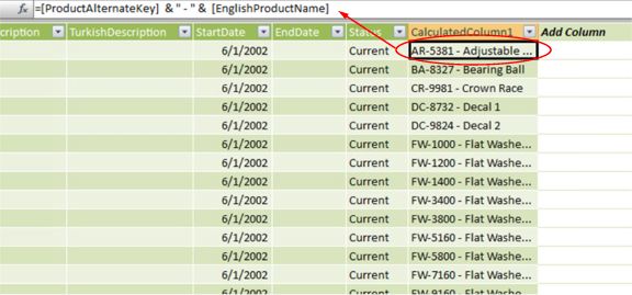
Illustration 11: The Newly Populated Calculated Column Appears …
We note that, upon creation of the calculated column, a new column is created to its immediate right, again with “Add Column” as its label, for easy addition of the next calculated column. Our new calculated column, containing the new combined Product label, is named CalculatedColumn1 by default. Let’s modify this to something more meaningful.
- Double click the column header of the newly added calculated column, currently containing the CalculatedColumn1 label.
- Type (or copy and paste) the following into the column heading:
ProductLabel
- Press the ENTER key.
The column header now displays the desired title.
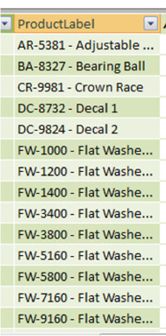
Illustration 12: The New Title Appears …
In our example above, we used the “&” operator to concatenate two columns, together with a text string in between. As we will see throughout the levels of Stairway to DAX, DAX provides many operators, which, with only a few exceptions, perform just like they do in Microsoft Excel. These operators include those shown in Table 1.
Operator | How Employed |
| Arithmetic Class | |
+ | Addition |
- | Subtraction (or negation) |
* | Multiplication |
/ | Division |
^ | Exponentiation |
| Parenthetic Class | |
() | Grouping / Precedence |
| Comparison Class | |
= | Equal to |
< | Less than |
<= | Less than or equal to |
> | Greater than |
>= | Greater than or equal to |
<> | Not equal to |
| Text Concatenation Class | |
& | Concatenation |
| Logic Operator Class | |
&& | And |
|| | Or |
! | Not / negation |
Table 1: DAX Operators
We will become familiar with these operators as we work through the levels of our series.
Next, as a prelude to moving into the core focus of our series, we’ll introduce DAX formulas and functions. We will then be ready to examine our first function.
DAX Formulas and Functions
We can exploit DAX formulas to create either calculated columns or measures. Let’s briefly introduce each of these “destinations” before kicking off the examination of our first function. We define calculated columns in the PowerPivot window, as we discovered in our last section. By contrast, we create measures within an Excel worksheet, where one or more pivot tables / charts reside which are supported by a PowerPivot table. The difference in where calculated columns and calculated measures are created is important to understand.
We create a calculated column from a PowerPivot window, either like we did above, by moving to and clicking the column with the header labeled “Add Column,” or by clicking the Add button in the Columns group within the Design ribbon. (We will create calculated columns via the Add button later.) Using either option, we input the DAX formula into the formula bar (by typing it, using Autosense, or a combination of both), as we did earlier, and then press ENTER. The PowerPivot Field List for any pre-existing pivot tables will notify us of changes in the underlying PowerPivot window, enabling a Refresh button we can use to update both the field list and the pivot table.
A measure is created from within an Excel workbook, within which a PivotTable / Pivot report must already exist. Once we have focus within the Pivot Table / report, or within the corresponding PowerPivot Field List, we can either right-click one of the tables in the field list or choose Add New Measure. Either action launches the Measure Settings dialog, as we shall see, into whose Formula text box we can input a desired DAX formula. We will get plenty of hands-on exposure to creating measures, as well as opportunities to learn about the importance of measure context, as we move through the levels of our series. For now, it’s enough to understand that we can use DAX formulas to create calculated columns and measures, and the basic differences between the two.
Next, let’s take a look at our first DAX function.
The RELATED Function
According to the Microsoft DAX Function Reference for PowerPivot, the RELATED() function “returns a related value from another table.”
The source column (“<column>”) is placed within the parentheses to the right of the word “RELATED,” as shown below:
RELATED(<column>)
The <column> placeholder represents the column containing the values that we wish to retrieve via the function. A single value related to the current row is returned. RELATED() requires that a relationship is in place between the current table (from which we are using the function) and the table with the related data. Using RELATED() we specify the column containing the desired data, and RELATED() traces the relevant relationship (many-to-one) to retrieve the value from the column we specify in the related table.
RELATED() performs a lookup, therefore, based upon the relationship in place, and examines all the values within the table we specify (ignoring any filters we have put in place, if applicable). A relationship must exist, of course, for the function to work. If there is no relationship, we have to create one to be able to use the function. (We work with relationships in other steps of our series, so we will become familiar with the straightforward process at a later time.) RELATED() works much like the Excel VLOOKUP() function, but is significantly more flexible in various ways. We will encounter various uses of RELATED(), often in conjunction with other DAX functions, throughout this series, where we will get a feel for the natural hierarchies it renders and so forth.
RELATED() can be used in a calculated column expression (the way we’ll work with it in this level), where the current row context is meaningful (we’ll talk about row context shortly). RELATED() can also be employed as a nested function within an expression using a table scanning function, which gets the current row value and then scans another table for instances of that value. (SUMX(), which we will examine early in the steps of this series, is one example of a popular table scanning function). RELATED() allows us to leverage relationships easily and transparently – and in a way that the information consumer is insulated from the underlying database components.
Let’s take a look at an example of the DAX RELATED() function at work within the AdventureWorksDW2008R2 sample we’ve established.
- Click the Design tab atop the PowerPivot window.
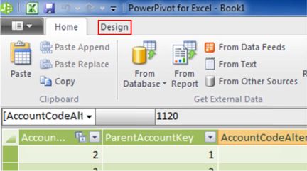
Illustration 13: The Design Tab atop the PowerPivot Window
- Click the Manage Relationships button on the Design tab, as shown.
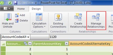
Illustration 14: The Design Tab atop the PowerPivot Window
The Manage Relationships dialog opens, and we see various relationships between tables that were defined within PowerPivot when we clicked the Select Related Tables button in our PowerPivot setup steps.
- Click the fifth row from the top in the table list of the dialog, labeled DimProduct [ProductSubcategoryKey], as depicted, to select it.
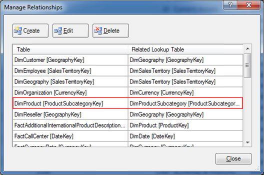
Illustration 15: Our Selection in the Manage Relationships Dialog
- Click the Edit button atop the dialog next.
The Edit Relationship dialog opens, and we are presented with the definition of the relationship between the DimProduct and DimProductSubcategory tables, as shown.
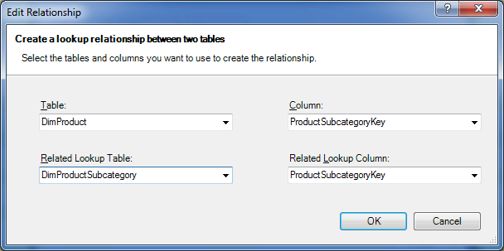
Illustration 16: The Edit Relationship Dialog …
The Edit Relationship dialog tells us that the related columns are DimProduct.ProductSubcategoryKey and DimProductSubcategory.ProductSubcategoryKey. We are therefore aware of the details of the relationship between the two tables via these columns. The existence of a relationship will allow us to use the RELATED() function in a way that we can be certain that the data it retrieves is accurate.
- Click OK to dismiss the Edit Relationship dialog.
- Click the Close button in the Manage Relationships dialog.
We return to the PowerPivot window – DimProduct tab. Now let’s get some exposure to the RELATED() function.
- Scroll over to, and click, the header of the column labeled Add Column, this time to the immediate right of the calculated column we added earlier, ProductLabel.
The Formula bar (fx) is activated, once again, upon selection of the column.
- Type (or copy and paste) the following into the Formula bar:
=RELATED(D
- Select the following from the Autosense-enabled selector that appears:
DimProductSubcategory[ProductSubcategoryAlternateKey]
as shown in this partial view:
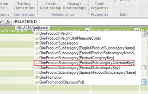
Illustration 17: Selecting a Column in a Related Table …
- Once the selection appears in the formula bar, add a right parenthesis symbol ( “ )” ) to close the expression, which will then appear in the formula bar as shown:
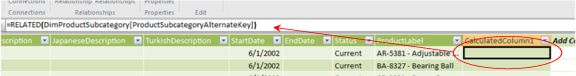
Illustration 18: The Completed Expression …
Note that we provide the table name before the column name, as the column resides in another table.
- Press the ENTER key.
The DAX formula containing the RELATED() function is accepted and the calculation populates the rows where a SubCategoryAlternateKey exists, leaving blank those where one does not (we can scroll down to see populated rows lower in the tab).
- Double click the column header of the calculated column, as we did with our first calculated column.
- Type (or copy and paste) the following into the column heading:
SubCatAltKey
- Press the ENTER key.
The column header now displays the desired title.
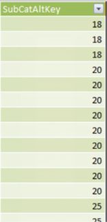
Illustration 19: The SubCatAltKey Calculated Column Appears …
Let’s add a couple more columns to reinforce our understanding of basic DAX formula creation and the RELATED() function.
- Click the column header labeled Add Column to the immediate right of the newly added SubCatAltKey calculated column.
- Type (use Autosense, or copy and paste, as desired) the following into the Formula bar:
=RELATED(DimProductSubcategory[EnglishProductSubcategoryName])
- Press the ENTER key, once again.
The DAX formula containing the RELATED() function is again accepted and the calculation populates the rows where an instance of EnglishProductSubcategoryName exists, leaving blank those where one does not, as before.
- Double click the column header of the newly added calculated column, once again.
- Type (or copy and paste) the following into the column heading:
SubCatName
- Press the ENTER key.
The column header now displays the desired title, as in previous steps.
Finally, let’s insert column to create a label combining the new SubCatAltKey and SubCatName columns in a manner similar to the way we created our first calculated column, ProductLabel.
- Click the column labeled Add Column to the immediate right of the newly added SubCatName calculated column.
- Type (or copy and paste, as desired) the following into the Formula bar:
= [SubCatAltKey] & " - " & [SubCatName]
- Press the ENTER key, once again.
The DAX formula containing the RELATED() function is again accepted and the calculation populates the rows, leaving only a solitary hyphen ( “-“ ) in the rows where the SubCatAltKey and SubCatName columns are empty.
- Double click the column header of the newly added calculated column, once again.
- Type (or copy and paste) the following into the column heading:
SubCatLabel
- Press the ENTER key.
The column header now displays the desired title, as in previous steps. The new calculated column appears, alongside the calculated columns combined to create it, as partially depicted (for a sample of populated rows) below.
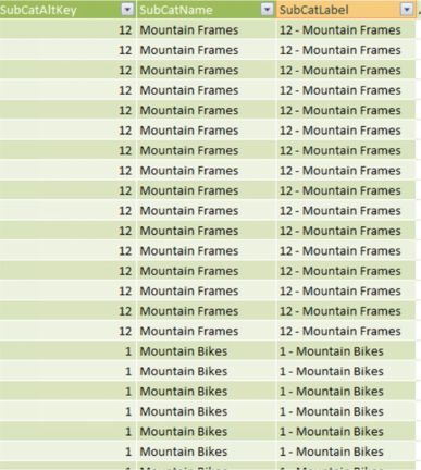
Illustration 20: The SubCatLabel Calculated Column Appears …
And so we see that our new calculated column delivers the desired results. Let’s save the PowerPivot work to date, along with spreadsheet with which it is associated.
- Using the downward pointing selector in the upper left corner of the PowerPivot window (to the immediate left of the Home and Design tabs), select Save As …, as shown.
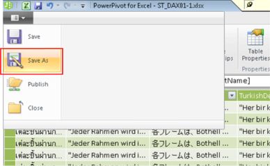
Illustration 21: Saving Our Work to Date …
- Name the file ST_DAX01-1.xlsx, and save it in a meaningful location.
- Exit Excel 2010 as desired.
We are now positioned to pull our PowerPivot data into Excel and perform analysis via a PivotTable, present data via a Pivot report, and so forth.
We will explore many functions, within the context of various formulas that we craft to meet representative business needs, as we move into subsequent steps’ coverage of DAX, and PowerPivot in general. A grasp of the functions, as well as agile practices surrounding the use of PowerPivot in query and modeling data, will be vital to success in our taking advantage of the vast opportunities that PowerPivot offers us. Practice with these components will assure that their use comes as second nature, and will create a foundation from which the power and elegance of PowerPivot can be fully exploited.
Summary …
With this article, I introduced the Stairway to PowerPivot and DAX series. I began by noting that the series is designed to provide hands-on introduction to the basics of PowerPivot and the Data Analysis Expression (DAX) language, with each level progressively exposing an individual function, technique or other component designed to help you to meet specific real-world needs. We noted that our primary objective within this series is to make those new to PowerPivot more comfortable with creating useful queries, within a business context, using the PowerPivot / DAX combination. Our means to that end will be to obtain hands-on exposure to using PowerPivot in general, while achieving an understanding of the DAX language, using formulas we construct from the DAX functions we introduce within the levels of this Stairways series.
For each function we introduce within the levels of the series, we will discuss what it is designed to produce and its operation in doing so, the syntax with which it is employed and the data that it retrieves and presents. I hope that this approach will encourage you to take the example code I present in the levels, and try it out, making changes and experimenting, so as to get the feel for the capabilities of DAX within PowerPivot. We’ll illustrate every point with practice examples of business uses along with useful queries.
In this, our first level of Stairway to PowerPivot and DAX, we introduced PowerPivot and DAX, discussing what you need to have in place to get started with the series. In preparation for the exercises to follow, we walked through the performance of an import, bringing in several tables from a sample SQL Server database that is readily available via sources we noted on the web. We next discussed DAX formulas and functions in general, and moved rapidly into our first exposure to DAX. We looked at the RELATED() function, and exposed a basic approach to using it in a simple scenario. Finally, we discussed the results we obtained from using the function in our practice examples, and looked forward to similar steps with the many DAX functions in future levels.