
In this Level we will introduce the MDX time / date series functions group. As we have discussed elsewhere in the Stairway to MDX series, many business requirements revolve around the performance of analysis within the context of time / date. In earlier levels, we saw simple approaches to meeting examples of these requirements (such as determining values for a prior, current, last, etc., reporting period) by using the .CurrentMember, .PrevMember and .NextMember functions, mainly because the time / date dimension provides an intuitive platform for the demonstration of many functions such as these.
Because of pervasive business requirement to analyze data within the context of time / date, MDX provides a specialized group of time / date series functions to meet these needs. In this Level, we will overview the PeriodsToDate() function, and then we will discuss the specialized “shortcut” functions that are based upon it, including YTD(), QTD(), MTD(), and WTD(). In subsequent steps, we will explore additional time / date series functions and expressions, together with other capabilities of MDX to help us to meet typical business needs.
Introducing the Time / Date Series Function
In performing virtually any type of data analysis with a cube, we become acquainted early on with the need to do so with reference to time / date. We might receive a request to compare revenue or expense across months, quarters, or years, for example. An information consumer might need to analyze growth over time or date periods, as another illustration. And common to any of us who have worked within accounting and finance circles is the requirement to present year-to-date totals, averages or other accumulations.
The time / date series functions are specifically designed to support time- or date -based analysis. They are largely applied to dimensions of the “time” or “date” type, but can be applied to other dimensions as well. We can use the time / date series functions to produce elaborate calculations and aggregations, some of which we will introduce in prospective levels as the Stairway to MDX progresses. Although, as an implementer, I have found different client environments to require differing numbers of levels within the time hierarchy (many accounting and financial scenarios have required that we present time down to the month level, but others have required the capability to report to the day, hour, minute, and even second levels), the time / date dimension within all of these environments has held one common attribute: the descendants of any given member in a time / date level are the same as the descendants of its peer levels. As an example, the descendants of the Calendar Year member 1997, in a typical scenario, are composed of Quarters 1 through 4, and Months January through December, while the descendants of peer Calendar Year member 1998 are identical.
The similarity in structure between members in a time / date dimension makes comparisons simple and efficient. The time / date series functions allow us to perform comparisons and other operations upon peer members that exist throughout the hierarchy (such as [Date].[Calendar].[Calendar Quarter].[Q3 CY 2006] and [Date].[Calendar].[Calendar Quarter].[Q3 CY 2008]), sequential members within a given level (such as the months indicated by [Date].[Calendar].[Month].[July 2006] and [Date].[Calendar].[Month].[August 2006], and other relationships based upon hierarchical similarities. Illustration 1 depicts these possibilities within the Adventure Works cube, housed within the Adventure Works 2012 SSAS Database.
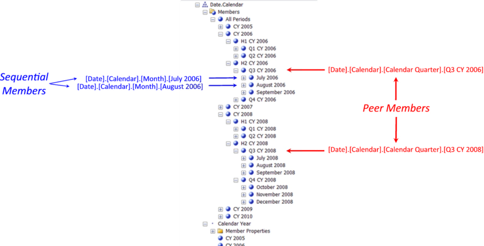
Illustration 1: Date.Calendar Hierarchy as Found in the Adventure Works Sample Cube (Partially Expanded)
In this Level we'll introduce the powerful PeriodsToDate() function, addressing various common considerations of time / date series functions as a part of our exploration. We will also reference other specialized time / date series functions that are based upon the PeriodsToDate() function. In introducing the PeriodsToDate() and related specialized functions, we'll examine the syntax surrounding, together with an illustrative example in a practice exercise of, the use of each. Throughout the steps we take within the practice session, we'll discuss the MDX results we obtain, as well as perform a review of the use of calculated members, primarily as a means of exploring the time / date series functions that we introduce within this Level.
The PeriodsToDate() Function
The PeriodsToDate() function, according to the Microsoft Developer Network, “returns a set of sibling members from the same level as a given member, starting with the first sibling and ending with the given member, as constrained by a specified level in the Time [ / Date] dimension.”
From another perspective, pointed a bit more in the direction of the Date dimension specifically (as the PeriodsToDate() function virtually always is, in my experience), PeriodsToDate() “returns a set of periods [members] from a specified level starting with the first period [sibling] and ending with a specified member.”
PeriodsToDate() returns the number of periods within the specified level, up to and including the specified member. If the level is specified the current member is inferred as Hierarchy.CurrentMember, where “hierarchy” represents the hierarchy of the specified member. When neither level nor member is specified, the inferred level is the parent level of the current member of the first hierarchy of the type Time in the relevant measure group. The Type setting can be determined by examining the Properties pane for the dimension – “Date” in the Adventure Works cube of the Adventure Works 2012 SSAS database sample, (seen from the Dimension Structure tab within the Date dimension) in SQL Server Data Tools (“SSDT”), as shown:
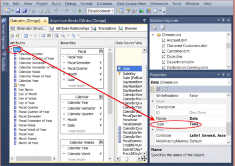
Illustration 2: Dimension Type Property Set to “Time” for the Date Dimension as Found in the Adventure Works Sample Cube (Partially Expanded)
Putting PeriodsToDate() to work is straightforward, once we grasp its general syntax and operation. PeriodsToDate() allows us to meet very common business needs where the concept of time / date is involved. An example is the calculation of a year-to-date total. The calculation of this total requires accumulation over a range of members of the Time / Date dimension. This set of time / date members is easily assembled using the PeriodsToDate() function, although other, less direct approaches exist to meet this requirement. (We will discuss the most common group of such approaches, shortcuts designed in MDX especially for this purpose – later in this Level, once we have examined the underlying PeriodsToDate() function.)
Syntactically, two arguments are placed within the parentheses to the right of PeriodsToDate, as shown here:
PERIODSTODATE( [ Level_Expression [ ,Member_Expression ] ] )
The function returns the number of member periods within the Level_Expression (a valid MDX expression that generates a level), up to and including Member_Expression. The following example expression would return the first six months of year 2008:
PERIODSTODATE(
   [Date].[Calendar].[Calendar Year],
      [Date].[Calendar].[Month].[June 2008]
   )
The members returned using the above expression within a query would be the same as those returned using the following range expression:
[Date].[Calendar].[Month].[January 2008]:[Date].[Calendar].[Month].[June 2008]
In the above, much as we see in other languages, the colon operator denotes a range; in our case, the range is members of the Date dimension, Year 2008, Month level of the Calendar hierarchy, members 1 (January) through 6 (June).
Let's extend the above function into a working example, using, as we commonly do, a calculated member as the means to our ends. As we've seen in Stairway to MDX - Level 10: “Relative” Member Functions: .CurrentMember, .PrevMember, and .NextMember, as well as elsewhere within our series, a calculated member is an excellent vehicle for familiarizing ourselves with the syntax, together with the dataset that it delivers.
/*  SMDX011-000-Example:  Employ PERIODSTODATE() function in a calculated
    Member to perform simple aggregation of a measure over date ranges  */WITH
MEMBER
   [Date].[Calendar].[2008_1st_Half] AS
       AGGREGATE(
           PERIODSTODATE(
              [Date].[Calendar].[Calendar Year],
              [Date].[Calendar].[Month].[June 2008]
           )
       )
SELECT
    {[Date].[Calendar].[2008_1st_Half]} ON 0,
    {[Product].[Category].CHILDREN} ON 1
FROM
    [Adventure Works]
WHERE
   [Measures].[Internet Sales Amount]
The dataset returned would appear as depicted:
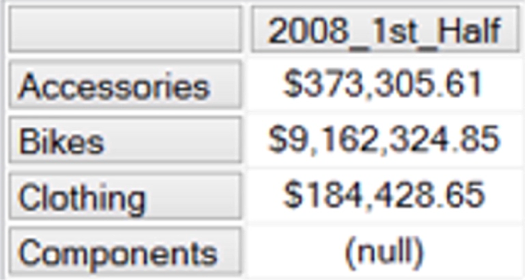
Illustration 3: Example Result Dataset Using the PeriodsToDate() Function
To summarize the action above briefly: the WITH section contains the definition of the calculated member / measure 2008_1st_Half. The PeriodsToDate() function is used, together with, and within the context of, the AGGREGATE() function; all are used within the definition of the calculated member. Let's “parse” the action here into plain English, as the combination we see above is certainly typical enough in the real world.
In delivering the aggregation of a numeric expression evaluated over the specified set, the syntax of the AGGREGATE() function is relatively straightforward, and might be represented as follows:
AGGREGATE(Set_Expression [ ,Numeric_Expression ])
The month range of the first semester of Calendar Year 2008 inhabits the Set Expression portion of the Aggregate() function. The Set Expression portion of the function supports the column axis within the returned dataset, via our calculated member 2008_1st_Half. We ask for members from the Date dimension (Calendar hierarchy) to populate our columns thereby; similarly, we ask for Product dimension (Category hierarchy) members to populate our rows axis.
We specify no measure within either axis, but, via the WHERE clause, we slice the data by the Internet Sales Amount, and thereby filter the data grid for that specific measure only. Because we used the Aggregate() function as the basis for accumulation within 2008_1st_Half, the juxtaposition of that calculated member with the measures delivers the desired aggregation of the measures across months January through June of 2008, thanks to the operation of PeriodsToDate().
Let's begin our hands-on exposure to PeriodsToDate(), to reinforce our understanding of the basics we have covered so far. We will, as usual, work with the MDX Query Editor in SSMS, as our tool for constructing and executing the MDX we examine, and for viewing the result datasets we obtain. If you are not sure how to set up SSMS in Analysis Services, see Stairway to MDX - Level 1: Getting Started with MDX,” where we detail the steps in a manner that will be largely identical for SSAS 2008R2 and above.
We'll begin with an illustration that employs PeriodsToDate() in a rudimentary way to demonstrate its basic operation: To provide a simple business need, let's say that a representative of our hypothetical client, Adventure Works Cycles, has asked that we generate a total of “valid” (translate: “non-empty”) resales activity for months preceding a specified month in a given year of operations (in this case, Calendar Year 2005).
- Click / select the Adventure Works cube in the SQL Server Management Studio (“SSMS”) Object Explorer.
- Click the New Query button above the Object Explorer.
- Type (or copy and paste) the following query onto the new canvas of the Query pane that opens:
-- SMDX011-001 Use PeriodsToDate() to generate valid "preceding periods" (second parameter is range limit)
SELECT

NON EMPTY {PERIODSTODATE(
            [Date].[Calendar].[Calendar Year],
[Date].[Calendar].[Month].[December 2005]
)} on 0,
{[Product].[Product Categories].[Category]} ON 1
FROM
    [Adventure Works]
WHERE
([Measures].[Reseller Sales Amount])
The Query pane appears, with our input.
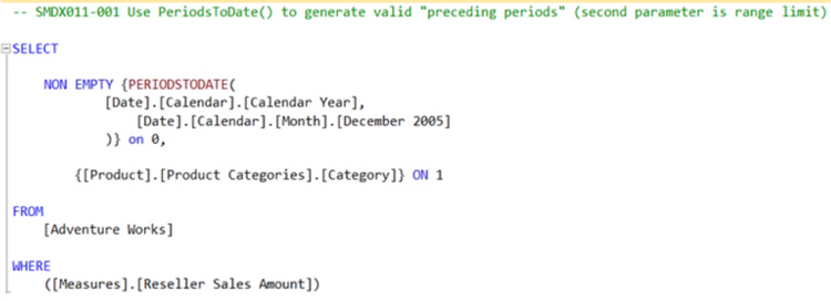
Illustration 4: Initial Practice Query, Employing PeriodsToDate(), in the Query Pane
- Click the Execute (!) button in the toolbar.
The Results pane is populated by Analysis Services, and the dataset appears, as partially shown.
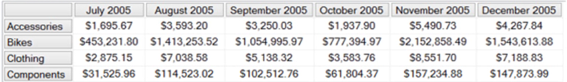
Illustration 5: Example Result Dataset Using the PeriodsToDate() Function
In the dataset returned above, we see every month that is populated within Calendar Year 2005 (the first of the two parameters of the PeriodsToDate() function, beginning with July (the first month containing a value) and continuing through (and including) December 2005. I chose a year with results only recorded in the last six months, as I reasoned that this would demonstrate that, for Calendar Year 2005 I would return the populated months preceding, and up to, the last month member in the time range specified in the second parameter of the PeriodsToDate() function.
- Save the query by selecting File Save MDXQuery1.mdx As …, naming the file SMDX011-001.mdx, and placing it in a meaningful location.
Let's get some more hands-on exposure with PeriodsToDate(), this time in a fresh application of what we have learned. Let's say that another AdventureWorks client colleague approaches us with a relatively common requirement: He wants to see a simple demonstration of how we might create a “running total” within a report that returns sales totals for each of several successive periods. For purposes of the demo, we obtain confirmation from our colleague that he'd like to see, for each of Calendar Years 2005 through the last year existing in our current cube structure, the corresponding total Internet Sales Amount. To the right of the column containing the Internet Sales Amount, he wishes to see a calculation named simply “Running Total Sales,” which accumulates, each year, the total of all years' sales before a given year, plus the current year, into the displayed respective running total.
- From our current position within the Query Editor, select File New from the top menu.
- Select Query with Current Connection from the cascading menu that appears next, as shown.
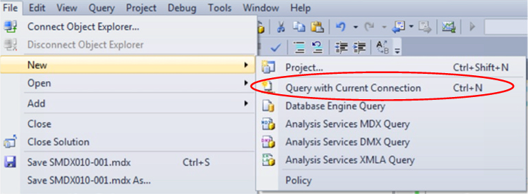
Illustration 6: Creating a New Query via the Current Connection
- Type (or copy and paste) the following query into the Query pane:
-- SMDX011-002 Use PeriodsToDate() to generate a "running total"
WITH
MEMBER
   [Measures].[Running Total Sales] AS
       SUM(
        PERIODSTODATE(
            [Date].[Calendar].[(All)],
            [Date].[Calendar].CURRENTMEMBER),
[Measures].[Internet Sales Amount]
)
SELECT
    {[Measures].[Internet Sales Amount], [Measures].[Running Total Sales]} ON 0,
    {[Date].[Calendar Year].CHILDREN} ON 1
FROM
    [Adventure Works]
The query appears within the Query pane:
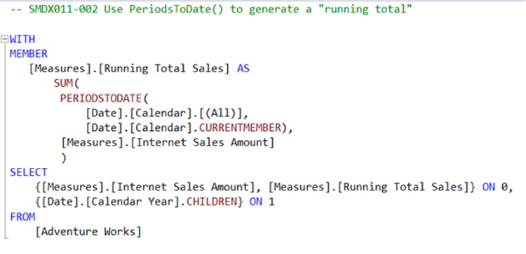
Illustration 7: Query Employing PeriodsToDate() Appears in the Query Pane
- Click the Execute (!) button in the toolbar, once again.
Analysis Services populates the Results pane, as partially shown:
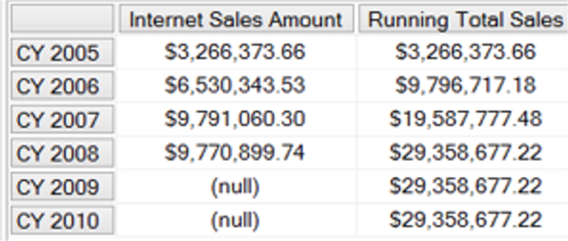
Illustration 8: The Query Results, “Running Total” Delivered via the Combination of PeriodsToDate() and .CurrentMember
The logic we employ in our calculated member, Running Total Sales, relies upon the combination of PeriodsToDate() and .CurrentMember. The latter, of course, is to specify the current member of the Calendar hierarchy, Year level of the Date dimension. Based upon the current member, we specify the second argument of the PeriodsToDate() function, dynamically extending the number of months (over the range between the first populated month in the year to the month corresponding to the month member stipulated in the rows axis, to the current member as the range endpoint) over which the summing of Internet Sales occurs.
- Save the query by selecting File Save MDXQuery2.mdx As …, naming the file SMDX011-002.mdx, and placing it, as we did with the query we constructed earlier, in a meaningful location.
Next, we'll extend our practical exposure to the PeriodsToDate() function to generate an approach to a similar, yet somewhat different, common business need. Let's say that our client colleague expresses satisfaction with the solution we have proposed immediately above, and next extends his request to the derivation of a similar calculation – but one that “resets” for each new year. That's right – he wishes to generate a “running total” within the context of each year; we commonly refer to this as a “year-to-date” total.
We'll start with a fresh scenario to illustrate this, this time using the calendar weeks level of the Date dimension, to make the display a little richer. This time, we'll pull in Reseller Sales for each week (limiting the rows axis to the weeks in 2007, to make the retained dataset more manageable) contained within the sample cube to demonstrate how to add a Year-to-Date (“YTD”) total calculation in a column to the right of the base measure. (I will indicate that this is a “longhand” version of the YTD calculation here, as I intend to demonstrate a “shorthand” version later.)
- From our current position within the Query Editor, select File New from the top menu, as we did earlier.
- Select Query with Current Connection from the cascading menu that appears next, once again.
- Type (or copy and paste) the following query into the Query pane:
-- SMDX011-003 Use PeriodsToDate() to generate a "longhand" YTD calculation
WITH
MEMBER
   [Measures].[YTD Resales ("Longhand")]
AS
   SUM(
        PERIODSTODATE(
            [Date].[Calendar Weeks].[Calendar Year],
               [Date].[Calendar Weeks].CURRENTMEMBER),
[Measures].[Reseller Sales Amount]
)
SELECT
    {[Measures].[Reseller Sales Amount],  [Measures].[YTD Resales ("Longhand")]} ON 0,
{[Date].[Calendar Weeks].[CY 2007].CHILDREN} ON 1
FROM
    [Adventure Works]
The query appears within the Query pane:
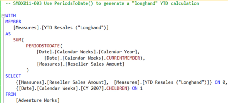
Illustration 9: Another Query, Employing PeriodsToDate(), Appears in the Query Pane
- Click the Execute (!) button in the toolbar, once again.
Analysis Services populates the Results pane, as partially shown:
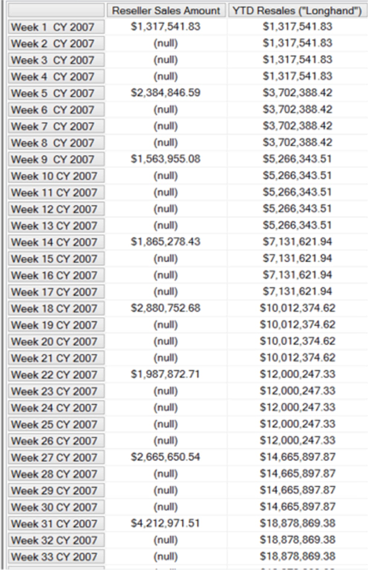
Illustration 10: The Query Results, “YTD” Delivered via the Combination of PeriodsToDate() and .CurrentMember (Partial View)
Within our calculated member, YTD Resales (“Longhand”), we rely once again upon the combination of PeriodsToDate() and .CurrentMember. The latter, of course, is employed to specify the current member of the Calendar Weeks hierarchy of the Date dimension. We therefore provide the second argument of the PeriodsToDate() function, which allows us to dynamically extend the number of weeks (over the range of the first week of the year to the week corresponding to the week member stipulated in the rows axis) over which the summing of Reseller Sales occurs. The year is, of course, physically limited to Calendar Year 2007, as we specify only the children (via the .Children function) of that year within our rows axis specification.
- Save the query by selecting File Save MDXQuery3.mdx As …, naming the file SMDX011-00.mdx, and placing it, once again, in a meaningful location.
Now that we've seen how to use the PeriodsToDate() function, let's take a look at the “shortcut functions” that derive from PeriodsToDate().
The PeriodsToDate() Shortcut Functions
As we have learned, the PeriodsToDate() function is used within the following basic syntax:
PERIODSTODATE( [ Level_Expression [ ,Member_Expression ] ] )
Several “shortcut functions” are available in MDX to allow us to perform time- / date-based summaries on corresponding period-to-date levels. Among these levels are the following, displayed in Table 1, that correspond to common levels of measurement in the business environment, together with the associated, specialized shortcut function that exists in MDX. For each of these “shortcut functions,” the Type property of the attribute hierarchy on which the level is based is set to the corresponding hierarchy level in the attribute design, as noted in the far-right column of the of the table.
| Level of Measurement | Shortcut Function | Attribute Hierarchy “Type” Property Setting |
| Year-to-Date | YTD() | Years |
| Quarter-to-Date | QTD() | Quarters |
| Month-to-Date | MTD() | Months |
| Week-to-Date | WTD() | Weeks |
Table 1: The PeriodToDate() Shortcut Functions
The shortcut functions named in Table 1 are each equivalent to the PeriodsToDate() function, with the appropriate levels (first argument) fixed for the specialized context within which each might be used. A composite of the syntax that each uses in the sample cube is as follows:
PERIODSTODATE( [Year] | [Quarter] | [Month] | [Week] [ ,Member_Expression ] )
Because the syntax is similar to all the shortcut functions, and because the operation of each is identical, with the exception of the specific levels involved, we will examine one sample of the group to confirm our understanding of general concepts. To this end, let's examine the QTD() function specifically.
The QTD() “shortcut” function defines the Level_Expression of the PeriodsToDate () function, upon which it is derived, to be Quarter. If no member is specified, the default is .Hierarchy.CurrentMember. In short, therefore:
QTD( [ Member_Expression ] )
is equivalent to
PERIODSTODATE (Quarter_Level_Expression, ] [ ,Member_Expression ] ).
The QTD() function serves as an “abbreviation” for the PeriodsToDate () function, where the Type property of the attribute hierarchy on which the level is based is set to Quarters, as depicted.
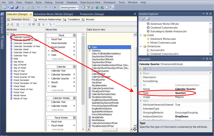
Illustration 11: Type Property for the Calendar Quarter Attribute Hierarchy Set to “Quarters” (Partially Expanded)
The QTD() function, along with the other PeriodsToDate() shortcut functions, relies upon the Type property for the Date hierarchy level appropriate to the shortcut (for QTD, as seen, it is “Quarters”), so it's a great idea to verify these settings in our Date dimensions as a part of overall SSAS Multidimensional best practices.
Let's practice with the QTD() function, via calculated member, in a manner that assists us in activating the concepts we've discussed. We'll assume, in this case, that our hypothetical client colleague, to whom we have imparted an understanding of the rudiments of the PeriodsToDate() function in the examples above, wishes to see an example of a shortcut function in action. We will respond to his request by rejoining the query editor in SSMS, and employing the QTD() function to return the aggregation of a base measure over a couple of months within a specified quarter.
From our current position within the Query Editor, select File New from the top menu, as we did earlier.
- Select Query with Current Connection from the cascading menu that appears next, once again.
- Type (or copy and paste) the following query into the Query pane:
/*  SMDX011-004 Use QTD() shortcut function to return the Order Quantities achieved, by Promotion, aggregated over the first two months of the third quarter of calendar year 2007 */WITH
MEMBER
   [Date].[Calendar].[Initial2Months2007] AS
       AGGREGATE(
           QTD([Date].[Calendar].[Month].[February 2007]
   )
       )
SELECT
    {[Date].[Calendar].[Initial2Months2007]} ON 0,
    NON EMPTY {[Promotion].[Promotion].CHILDREN} ON 1
FROM
    [Adventure Works]
WHERE
    ([Measures].[Reseller Order Count])
The query appears within the Query pane:
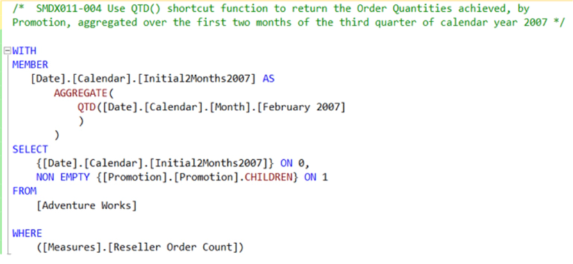
Illustration 12: Query Employing PeriodsToDate() “Shortcut,” QTD(), Appears in the Query Pane
- Click the Execute (!) button in the toolbar, once again.
Analysis Services populates the Results pane, with the following results:
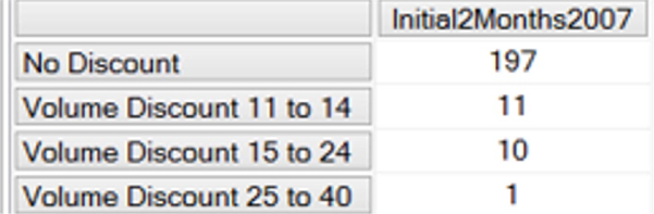
Illustration 13: The Query Results, “QTD” Aggregation of January and February of 2007
Within our calculated member, Initial2Months2007, we employ the QTD() function to return the Order Quantities measure for the first two months in Calendar Year 2007. As we noted in our initial explanation of the “shortcut” functions, QTD() “defines the Level_Expression of the PeriodsToDate () function, upon which it is derived, to be Quarter.” In the syntax of its use, the “QTD” portion of “ QTD( [ Member_Expression ] ) “ is equivalent to “ PERIODSTODATE (Quarter_Level_Expression ] “, so “PERIODSTODATE (Quarter_Level_Expression ]” is effectively the “hardcoded” identity of “QTD,” and is followed by the Member_Expression argument of [Date].[Calendar].[Month].[February 2007].
We simply juxtapose the child members of the Promotion hierarchy of the Promotion dimension (behind the NON EMPTY keyword, to suppress nulls) with the new calculated member, and we obtain the quarter-to-date aggregation of the first two months in Calendar Year 2007.
- Save the query by selecting File Save MDXQuery4.mdx As …, naming the file SMDX011-4.
We can easily confirm the accuracy of our numbers results with the following query:
-- SMDX011-005 Confirmation of accuracy of QTD calculation in SMDX011-004
SELECT
    {[Date].[Calendar].[Month].MEMBERS} ON 0,
    {[Promotion].[Promotion].CHILDREN} ON 1
FROM
    [Adventure Works]
WHERE
    ([Measures].[Reseller Order Count])
Once Analysis Services returns the resulting data set, we can scroll over to the columns representing January and February of 2007, and visually verify that the values of the two, added together, give us the values delivered by our new Initial2Months2007 calculation, as shown.
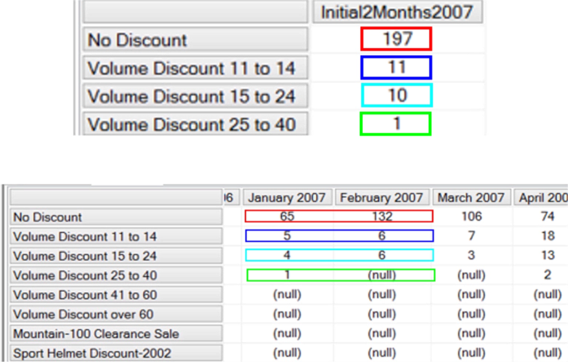
Illustration 14: Verification of Accuracy of the New Calculated Member (Partial, Composite View)
The remaining “shortcut” functions behave in a similar manner to QTD(), of course. We can easily see the utility of the shortcut functions for cases where the Level_Expression argument, such as Quarter in our last example, is predefined.
- Save the “verification” query, if desired, to a convenient location.
- Exit SSMS as desired.
PeriodsToDate(), together with its derivative “shortcut” functions, are truly staples within the MDX toolset. Moving into subsequent Levels of Stairway to MDX, and into progressively more advanced stages of query building, we will call upon these functions often to achieve aggregations and other effects involving the Time / Date dimension. As we'll see, they are often quite powerful when used in tandem with other functions. A grasp of these robust, flexible functions will be vital to success in our taking advantage of the more complex MDX concepts that we encounter in the business world. Practice with these components will assure that their use comes as second nature to us, and will create a foundation from which the power and elegance of MDX can be fully exploited.
Summary…
In this Level, we began an introduction to the time / date series functions group, noting that many business requirements revolve around the performance of analysis within the context of time / date. We started with an overview of the pervasive PeriodsToDate() function, and then we discussed the specialized “shortcut” functions that are based upon it, including YTD(), QTD(), and MTD(). We obtained familiarity with the purposes and uses of these functions, discussing the syntax within which they are used, as well as the information they return and other details.
We gained the know-how needed to take advantage of these useful functions through the typical Stairway to MDX practice exercises, whereby we constructed queries that used each function, and then examined the results datasets those queries delivered. Throughout the Level, we laid the foundation for our continuing examination of other time / date series functions and expressions, together with other capabilities of MDX to help us to meet typical business needs.