Disk and CPU related performance counters and DMV information can be difficult to interpret and compare when activity levels differ massively. This Cellular Automation (CA) application places a precise workload that can be repeated, measured and observed. It includes various ‘Pattern Generators’, one that uses Geometry and places a CPU load, another that uses set based queries that are IO bound and another ‘Hekaton’ version that uses in-memory tables and stored procedures. All 3 are mathematically provable implementations of ‘Conway’s Game of Life’, and an effective way to benchmark and compare the relative performance of different SQL Servers.
Benchmarking Process Overview
Step 1 – Initialization – An ‘Initialize’ procedure clears down any historic patterns associated with the calling session then populates a ‘Merkle’ table with the coordinates for an initial set of new patterns. Differing initial pattern complexity levels can be set using a ‘Stress Level’ parameter:
| Initial Patterns | Procedure Call |
| A simple 3 Merkle pattern that oscillates between 2 cycles | EXECUTE dbo.CA_InitPatterns @StressLevel = 1; |
| 4 Oscillating patterns including a complex 3 cycle ‘Pulsar’ | EXECUTE dbo.CA_InitPatterns @StressLevel = 1; |
| 4 Oscillating patterns and 2 ‘Gosper Glider Gun’ patterns described in the appendix | EXECUTE dbo.CA_InitPatterns @StressLevel = 3; |
Step 2 -Stress Testing – The ‘Pattern Generator’ procedures create the number of new patterns specified in a parameter, they use different techniques that stress different areas of a SQL instance. The Merkle table holds all patterns generated for a specific session, multiple calls can be made to the pattern generators from different sessions, each session maintains its own state.
| Compatibility | Procedure Call |
| SQL Server 2005 or higher | EXECUTE dbo.CA_GenPatterns @NewPatterns = 100, @Generator = ‘IO’ |
| SQL Server 2008 or higher | EXECUTE dbo.CA_GenPatterns @NewPatterns = 100, @Generator = ‘CPU |
| SQL Server 2014 or higher | EXECUTE dbo.CA_GenPatterns @NewPatterns = 100, @Generator = ‘HEK’ |
Step 3 – Results Verification – The ‘Display Pattern’ procedure shows the highest generation of patterns for the current session. The geometry data type is used to visualize the patterns, to confirm the final pattern and check for successful completion.
| Display Patterns | Procedure Call |
| Hekaton In-memory Merkles | EXECUTE dbo.CA_DspPatterns_SQL; |
| Disk based table Merkles | EXECUTE dbo.CA_DspPatterns_Hekaton; |
There's no learning curve involved in using this application and no client tools to install on your network, simply run one of the T-SQL setup scripts then execute a test, concurrently in multiple query analyser sessions if necessary. Change the 'Test' variable at the top to indicate the scenario being run, it's used later for comparing results.
Benchmarking Example - Physical / Virtual Server Performance Comparison
The CPU, IO and in-memory performance of the 2 servers below are compared in this example. Both are SQL Server 2014 instances with SP1, maximum memory set to 8 GB and default parallelism. Background activity was minimized by stopping other SQL instances and all SQL Agent services.
Physical Server (PHY)
- OS Name: Microsoft Windows Server 2012 Standard
- OS Version: 6.2.9200 N/A Build 9200
- System Manufacturer: HP
- System Model: ProLiant ML110 G6
- System Type: x64-based PC
- Processor(s): 1 Processor(s) Installed. [01]: Intel64 Family 6 Model 30 Stepping 5 GenuineIntel ~2394 Mhz
- Total Physical Memory: 8 GB
Virtual Server (VM
- OS Name: Microsoft Windows Server 2012 R2 Standard
- OS Version: 6.3.9600 N/A Build 9600
- System Manufacturer: Microsoft Corporation
- System Model: Virtual Machine
- System Type: x64-based PC
- Total Physical Memory: 8 GB
The following tests were performed, VP represents Virtual Processors assigned to the VM, CR represents Concurrent Requests
Physical Server
- PHY – 4 PR – 1 CR – 8 GB
- PHY – 4 PR – 2 CR – 8 GB
- PHY – 4 PR – 4 CR – 8 GB
Virtual Server 4 Virtual Processors
- VM – 4 VP – 1 CR – 8 GB
- VM – 4 VP – 2 CR – 8 GB
- VM – 4 VP – 4 CR – 8 GB
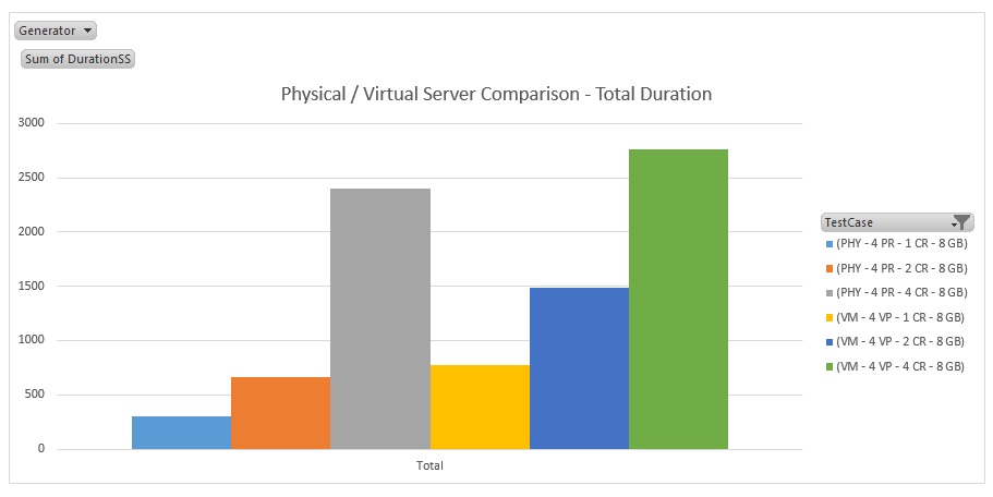
Between each test, the CA setup script was rerun to drop and recreate the database. The ‘Duration’ is the total time (microseconds) taken by the different pattern generators to produce 100 new patterns, lower represents faster processing times. The T-SQL script below was executed after the CA 2014 setup script to simulate a load.
USE [CellularAutomation]
GO
DECLARE @RC int;
DECLARE @Batches_IO int = 10;
DECLARE @Batches_CPU int = 10;
DECLARE @Batches_Hekaton int = 10;
DECLARE @NewPatterns int = 100;
DECLARE @TestCase varchar(50) = 'VM - 1 VP - 4 CR - 8 GB';
DECLARE @StressLevel int = 3;
EXECUTE @RC = [dbo].[CA_LoadTestExecute]
   @Batches_IO
  ,@Batches_CPU
  ,@Batches_Hekaton
  ,@NewPatterns
  ,@TestCase
  ,@StressLevel;
GO
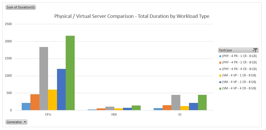
The resulting graphs below show a comparison between the Virtual and the physical server processing time for this same precise, exactly the same workload. Overall and by workload type. The physical Server is faster at processing CPU, IO and Hekaton workload types.
Benchmarking Example - Hekaton OLTP / OLAP Performance Analysis
Microsoft released a whitepaper recently titled ‘In-Memory OLTP – Common Workload Patterns and Migration Considerations’. In it they show how Hekaton performance varies in comparison with traditional SQL Server tables and procedures, and the workload patterns that suit in-memory OLTP. While not disputing the Microsoft whitepaper, it doesn’t include code samples to support the points made, this article does.
This test workload pattern shows that Increasing index sizes and logical reads have a negative impact on Hekaton performance, but conversely the more procedure calls a second the better it performs in comparison with traditional SQL. It uses a Cellular Automation (CA) mathematical database application to place similar demands in Hekaton and a corresponding set of native SQL Server tables and stored procedures.
The test was performed in a single query analyser session so the Hekaton concurrency improvements aren’t considered, the CA application does support multiple concurrent sessions but they weren’t used. Even just the benefit of not having to compile and interpret queries makes a massive difference, 75 times faster in this reproducible test.
Execute the OLTP / OLAP Test Simulation
- First run the Cellular Automation SQL Server 2014 Stress Testing Application setup script
- Start PERFMON then run the ‘OLTP / OLAP Simulation’ script attached twice, once with @StressLevel set to 1 then again with it set to 3. When these have both finished then the test is complete so stop PERFMON.
OLTP / OLAP Spectrum Analysis and Conclusions
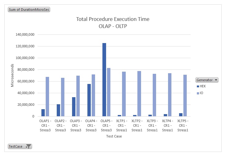
The simulation script varies the workload type as the test progresses, initially favouring OLTP but transitioning gradually to more of an OLAP bias. The ‘OLTP / OLAP Simulator’ script initially makes 512 procedure calls each requesting the generation of 1 new pattern (OLTP Bias), this slides across the OLTP / OLAP spectrum until finally 1 procedure call is made requesting the generation of 512 new patterns (OLAP Bias). The Pie Charts show how long each set of procedures took to complete the requests at different Stress Levels, notice Hekaton performance falling away relative to the native SQL ‘IO’ procedure as the cost of each call increases and the frequency of the calls decreases.
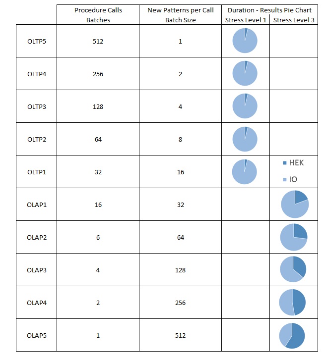
The difference in total execution times between Hekaton and SQL Server stored procedures and queries varies according to the batches called and the cost per batch. When the batch costs are low and frequent (XLTP below) then there are significant gains in using Hekaton, but as cost increases and frequency decreases (OLAP below) then the gains are gradually lost.
Stress Test Description
The OLTP / OLAP bias is heavily influenced by the ‘Stress Level’ parameter in the simulation test script which can be assigned a value of either 1, 2 or 3. The Cellular Automation application generates new patterns based on applying ‘cell comes alive’ / ‘cell dies’ rules to an initial starting pattern. The more complex the starting pattern, the more intensive the subsequent workload.
@StressLevel = 1 (Heavy OLTP Bias Workload)
The initial state includes one simple, 3 Merkle Pattern that oscillates between 2 states, there is very little work involved in constructing the next new pattern.
@StressLevel = 3 (Heavy OLAP Bias Workload)
Gosper Glider Gun patterns are created at Stress Level 3 which give birth to two new glider patterns once every 30th iteration, the workload and IO cost increase gradually as new patterns are created.
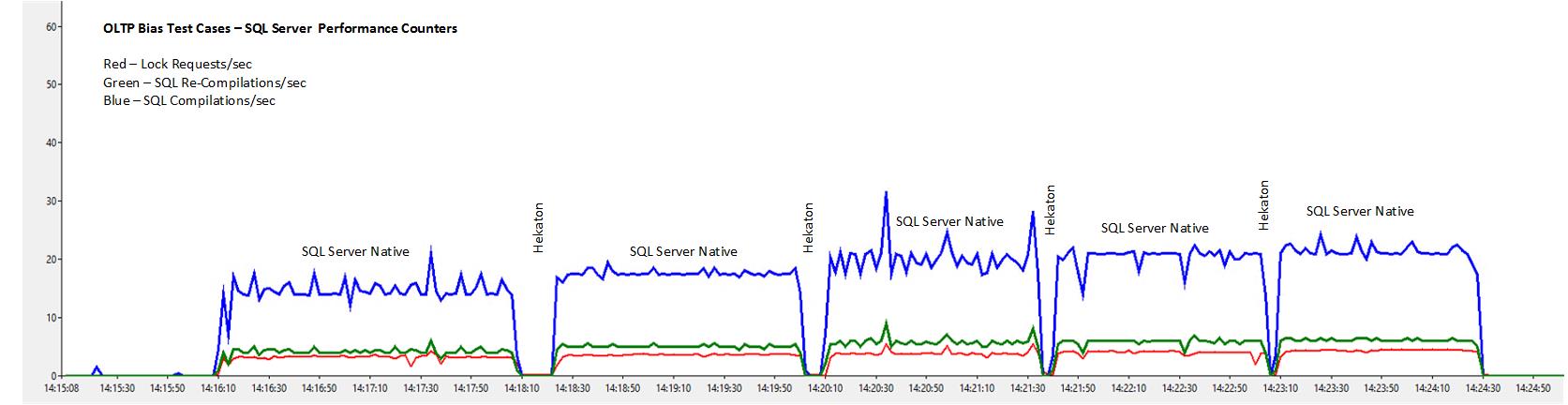
The Good – OLTP
Natively Compiled Stored Procedures.
When a procedure is called hundreds of times a second the savings from not having to compile or interpret T-SQL queries can be significant. The graph below shows the total duration of procedures calls for the SQL Server and Hekaton pattern generator stored procedures. Both performed exactly the same work (batch requests and batch size) using very similar queries and indexes, the results in the graph are filtered as below:
- Stress Level = 1
- OLTP 1 to 5 workloads
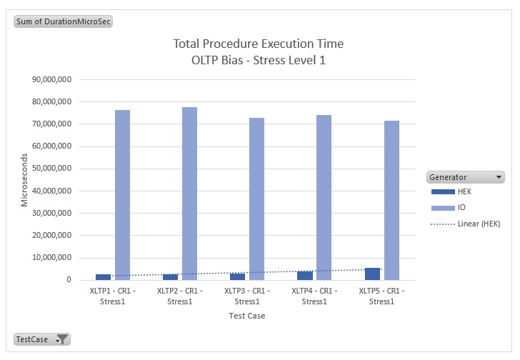
OLTP bias workloads are Hekatons strength, the total procedure execution time to perform a very similar workload is significantly lower than the corresponding interpreted SQL Server procedure calls using disk based tables. The graph below shows compilation and lock request counters during the OLTP bias test cases.
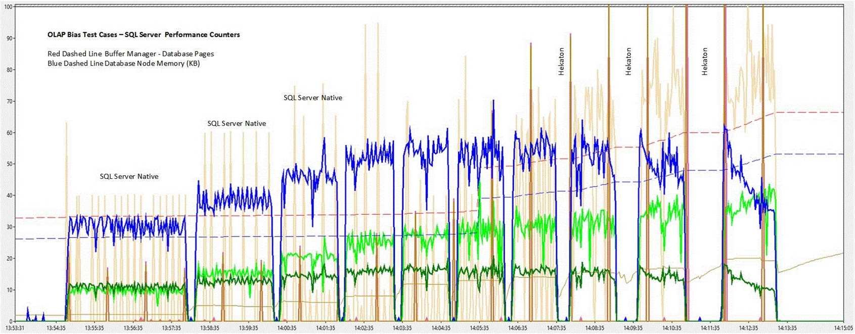
The Bad – OLAP
Performance deteriorates in Hekaton as the size of the indexes, and logical reads, increases. The graph below shows the total duration of procedures calls for the SQL Server and Hekaton pattern generator stored procedures. Both performed exactly the same work (batch requests and batch size) using very similar queries and indexes, the results in the graph are filtered as below:
- Stress Level = 3
- OLAP 1 to 5 workloads
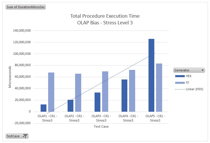
OLAP bias workloads are Hekatons weakness. Execution times deteriorate in comparison with SQL Server disk based tables and interpreted stored procedures performing the same workload, as the batch size increases. Memory usage also becomes an issue when processing larger indexes, ‘System out of memory’ errors become a risk.
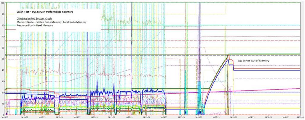
The Ugly – System Out of Memory
Request 1,000 new Hekaton Stress Level 3 patterns in 4 concurrent sessions and the error message below is typically shown after about 80 seconds. The only recovery I have found is to restart the SQL Service and the Hekaton database is in a recovery state for sometime after the instance comes back online. Data lose is typical although I haven’t researched it, an alternative table schema definition in the setup script might resolve this problem.
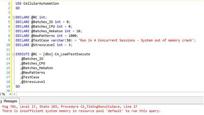
Performance Monitor showed ‘Memory Node – Stolen Memory, Total Memory’ and ‘Resource Pool – Used Memory’ counters all spiking just prior to the crash.
Benchmarking Example - Synthetic Transactions
This heading describes a simple framework for measuring SQL Server database application performance from both CPU & IO perspectives. A ‘Synthetic Transaction’ is proposed that is :
- Precise – A mathematical workload is performed the duration of which is measured. A 10 second test once every 10 minutes is sufficient for trend analysis.
- Easy to implement – There are no tools to install and no learning curve. Simply run the T-SQL setup script then schedule a SQL Agent Job.
- Flexible – The workload can be tuned for OLAP / OLAP bias and for the cost of execution.
- Unambiguous – The ‘duration’ measured is processing time for the same data, queries and plans.
The ‘cellular automation’ application generates new patterns according to a precise set of mathematical rules. It records the start and end time of each call which is a reflection on how SQL Server is handling client requests.
Test Process
Setup
Run the ‘CA Setup 2008’ script to create the cellular automation database application, then schedule a SQL Agent job for the steps below.
CPU Check Step
A call is made to the Cellular Automation engine requesting the generation of 200 ‘New Patterns’ at ‘Stress Level’ = 1. This calls the geometry intersects method which requires CPU, it runs for between 5 and 10 seconds’
IO Check Step
A call is made to the Cellular Automation engine requesting the generation of 100 ‘New Patterns’ at ‘Stress Level’ = 3. This calls set based queries which are IO bound, it runs for between 5 and 10 seconds’
Job Scheduling
A SQL Agent job to run both the CPU and IO check steps once every 10 minutes, an example of the T-SQL used for the job step is below:
-------------------------------
-- Use either the SQL Server 2008 - 2012 script below or the SQL Server 2014
-- depending on which version of the CA Setup script was used.
-------------------------------
USE CellularAutomation
GO
-- SQL Server 2008 / 2012 - SLA Synthetic Transaction IO Performance
DECLARE @RC int;
DECLARE @Batches_IO int = 1;
DECLARE @Batches_CPU int = 0;
DECLARE @NewPatterns int = 100;
DECLARE @TestCase varchar(50)  = 'SLA Synthetic Transaction - SQL IO' ;
DECLARE @StressLevel int = 3;
EXECUTE @RC = dbo.CA_LoadTestExecute @Batches_IO, @Batches_CPU, @NewPatterns, @TestCase, @StressLevel
GO
--  SQL Server 2008 / 2012 - SLA Synthetic Transaction CPU Performance
DECLARE @RC int;
DECLARE @Batches_IO int = 0;
DECLARE @Batches_CPU int = 1;
DECLARE @NewPatterns int = 200;
DECLARE @TestCase varchar(50) = 'SLA Synthetic Transaction - SQL CPU';
DECLARE @StressLevel int = 1;
EXECUTE @RC = dbo.CA_LoadTestExecute @Batches_IO, @Batches_CPU, @NewPatterns, @TestCase, @StressLevel
GO
-- Tidy preparation for next check, start empty for query plan reuse
TRUNCATE TABLE dbo.GridReference
TRUNCATE TABLE dbo.Merkle
GO
-------------------------------
-- OR
-------------------------------
USE CellularAutomation
GO
-- SQL Server 2014 - SLA Synthetic Transaction IO Performance
DECLARE @RC int;
DECLARE @Batches_IO int = 1;
DECLARE @Batches_CPU int = 0;
DECLARE @Batches_Hekaton int = 0;
DECLARE @NewPatterns int = 100;
DECLARE @TestCase varchar(50)  = 'SLA Synthetic Transaction - SQL IO' ;
DECLARE @StressLevel int = 3;
EXECUTE @RC = dbo.CA_LoadTestExecute @Batches_IO, @Batches_CPU, @Batches_Hekaton, @NewPatterns, @TestCase, @StressLevel
GO
--  SQL Server 2014 - SLA Synthetic Transaction CPU Performance
DECLARE @RC int;
DECLARE @Batches_IO int = 0;
DECLARE @Batches_CPU int = 1;
DECLARE @Batches_Hekaton int = 0;
DECLARE @NewPatterns int = 200;
DECLARE @TestCase varchar(50)  = 'SLA Synthetic Transaction - SQL CPU' ;
DECLARE @StressLevel int = 1;
EXECUTE @RC = dbo.CA_LoadTestExecute @Batches_IO, @Batches_CPU, @Batches_Hekaton, @NewPatterns, @TestCase, @StressLevel
-- Tidy preparation for next check, start empty for query plan reuse
TRUNCATE TABLE dbo.GridReference
TRUNCATE TABLE dbo.Merkle
GO
Test Results
The results below are from 2 Hyper-V virtual servers and a physical server described in the appendix. There was no concurrent client activity in any of the databases while these baselines were captured.
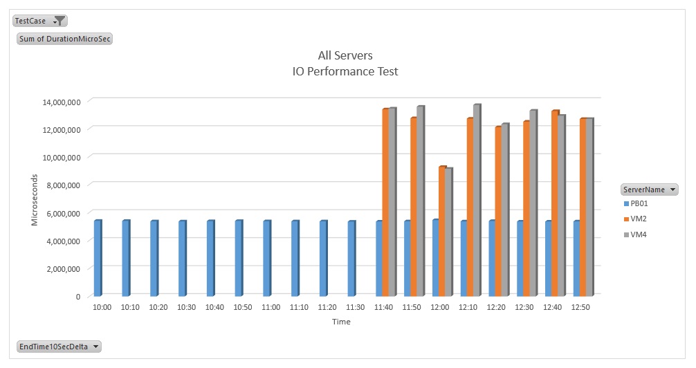
All Servers – IO Performance
The ‘Total Duration’ of calls to the SQL IO pattern generator shows a consistency and level of performance on the physical server that is not shared by either of the virtual servers.
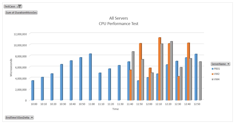
All Servers – CPU Performance
The baseline was started on the Physical Server 90 minutes before the virtual servers. CPU performance on the virtual servers is more volatile than the physical server.
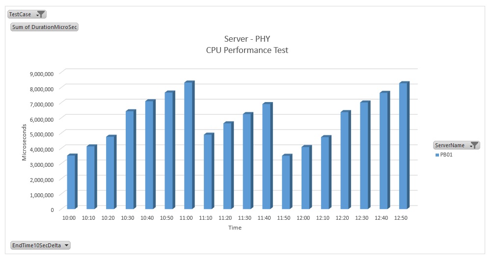
Physical Server – CPU Performance
The ‘Total Duration’ of calls to the CPU pattern generator show a clear trend on the physical server. Cross referencing the trend below against a baseline set of Windows Server and SQL Server performance counters would identify the cause, some sort of cache flushing looks likely.
Baseline Example Lab
These example results were from a simple environment consisting of 3 SQL Server 2014 SP1 instances:
One Physical Server (PB01)
- OS Name: Microsoft Windows Server 2012 Standard
- OS Version: 6.2.9200 N/A Build 9200
- System Manufacturer: HP
- System Model: ProLiant ML110 G6
- System Type: x64-based PC
- Processor(s): 1 Processor(s) Installed. [01]: Intel64 Family 6 Model 30 Stepping 5 Genuine Intel ~2394 Mhz
- Total Physical Memory: 8,192 MB
Two Virtual Servers – (VM2 & VM4)
- OS Name: Microsoft Windows Server 2012 R2 Standard
- OS Version: 6.3.9600 N/A Build 9600
- OS Manufacturer: Microsoft Corporation
- System Model: Virtual Machine
- System Type: x64-based PC
- Processor(s): 1 Processor(s) Installed.
- Total Physical Memory: 4,093 MB
The VM’s 2 and 4 are configured differently in Hyper-V, VM4 is using best practise settings for the following:
- Use Dynamic Memory
- Use fixed virtual hard disks for database files
- Generation Type 2 Virtual Machines
At such low levels of client activity, there were no discernable differences in performance between the 2 virtual servers.
Conclusions
- In specific circumstances, Hekaton is 75 (achieved with these scripts) or more times faster than native SQL procedures. Hekaton performance degrades in comparison with native SQL procedures though as the workload cost per batch increases and the frequency of batch requests decreases. As workload types become more OLAP bias, memory becomes an issue and performance deteriorates.
- Synthetic ‘Cellular Automation’ transactions offer a mathematically precise way to measure SQL Server database application CPU and IO performance at any given moment. A simple 5 second CPU & IO check once every 10 minutes could capture the performance information needed. Aggregated and potentially summarized across multiple servers for a given period it might provide a clear and unambiguous insight into database application performance.
Disclaimer
All of the pattern generators in this application will stress a SQL instance and are designed for isolated testing environments, you use them at your own risk.
References
- http://en.wikipedia.org/wiki/Conway’s_Game_of_Life – This Wikipedia link explains all the principles and patterns used in this article.
- https://www.simple-talk.com/sql/sql-training/the-sql-of-the-game-of-life/ – This ‘simple talk sql training’ article prompted this article.
- http://blog.sqlauthority.com/2015/04/29/sql-server-script-knowing-data-and-log-files-are-on-the-same-drive/ – Get default data folder for Hekaton file.
- ‘SQL Server Internals: In-Memory OLTP’ by Kalen Delaney
- https://msdn.microsoft.com/en-us/library/dn673538.aspx
- https://pal.codeplex.com/
- http://sqlperformance.com/2015/05/io-subsystem/analyzing-io-performance-for-sql-server
- https://www.simple-talk.com/sql/database-administration/hekaton-in-1000-words/
- https://msdn.microsoft.com/en-gb/library/dn170449.aspx
APPENDIX – Cellular Automation Mathematical Process and Proof
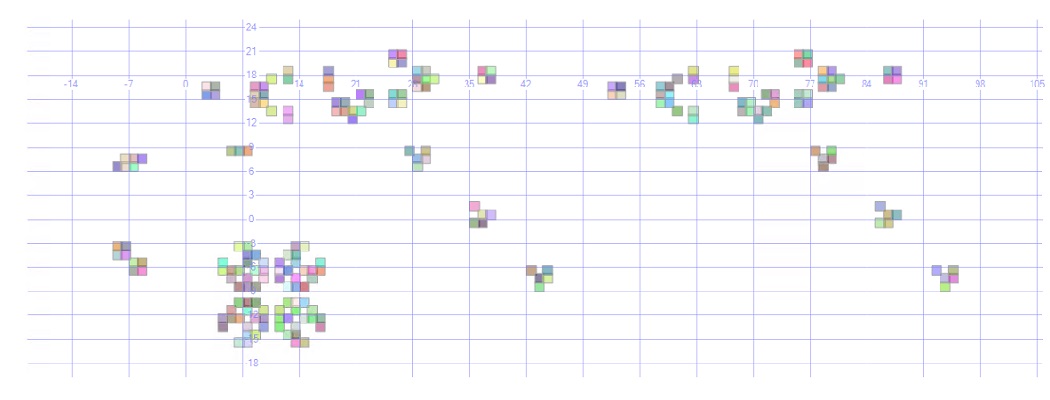
After running the CA Setup script, execute the ‘Initialize Patterns’ and ‘Display Patterns’ stored procedures to create and show Merkles in their initial state. Click on the ‘Spatial Results’ tab in SQL Server Management Studio to view as shown below.
USE CellularAutomation
GO
EXECUTE dbo.CA_InitPatterns @StressLevel = 2;
EXECUTE dbo.CA_DspPatterns_SQL;
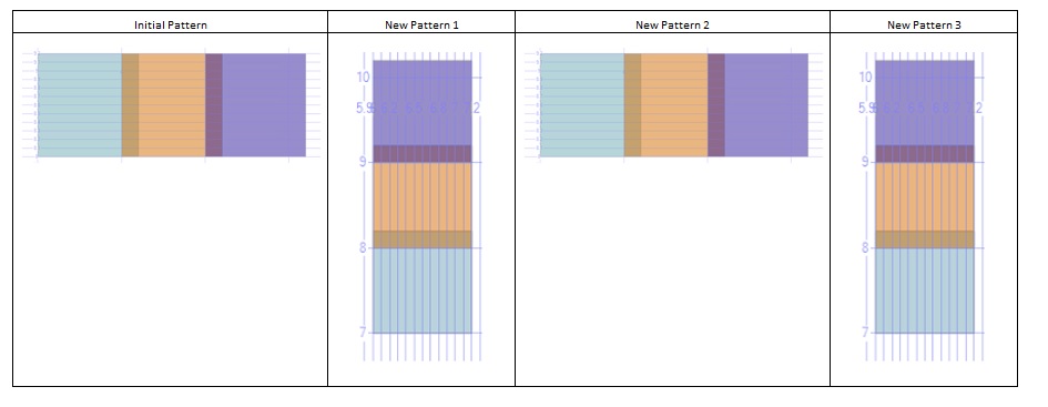
Now run the Pattern Generator stored procedure requesting the generation of 5 new patterns as below, each iteration is the result from applying Conway’s rules to the previous pattern. After 5 iterations the patterns differ to those at the start immediately after initialization, the oscillation cycle results in new patterns matching the initial pattern every 6th iteration.
EXECUTE dbo.CA_GenPatterns @NewPatterns = 5, @Generator = 'IO';
EXECUTE dbo.CA_DspPatterns_SQL;
The patterns cycle through their phases and match the initial pattern again every 6th iteration as illustrated below. Run the ‘Generate Pattern’ stored procedure 1 more time to complete the 6th cycle.
EXECUTE dbo.CA_GenPatterns @NewPatterns = 1, @Generator = 'IO';
EXECUTE dbo.CA_DspPatterns_SQL;
| New Pattern | 3 Oscillation Cycles (Pulsar) | 2 Oscillation Cycles (Blinker, Toad, Beacon) |
| 0 - Initiial Pattern | Cycle 1 | Cycle 1 |
| 1 | Cycle 2 | Cycle 2 |
| 2 | Cycle 3 | Cycle 1 |
| 3 | Cycle 1 | Cycle 3 |
| 4 | Cycle 2 | Cycle 1 |
| 5 | Cycle 3 | Cycle 3 |
| 6 | Cycle 1 | Cycle 1 |
This is the proof that this application meets all of Conway’s mathematical rules.
Mathematical Rules
In this application, Merkles are entities who’s existence at each iteration is as x and y axis coordinates, a ‘Merkle’ is a cell and a set together form a pattern.
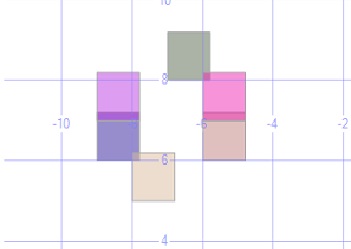
With the ‘CPU’ intensive pattern generator, these are converted to geometric polygons, cell sizes are increased by 20% and the geometric ‘Intersect’ method is used to count adjacent Merkles. This is illustrated in the ‘Toad’ pattern shown below in its base state/starting pattern.
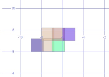
When the rules below are applied to the pattern above:
- Any live cell with fewer than two live neighbours dies, as if caused by under-population.
- Any live cell with two or three live neighbours lives on to the next generation.
- Any live cell with more than three live neighbours dies, as if by overcrowding.
- Any dead cell with exactly three live neighbours becomes a live cell, as if by reproduction.
The pattern below is generated on the 1st iteration, it returns to it’s base state/starting pattern on the next iteration, this pattern oscillates between 2 states.
Appendix – Stress Level 3 Workload
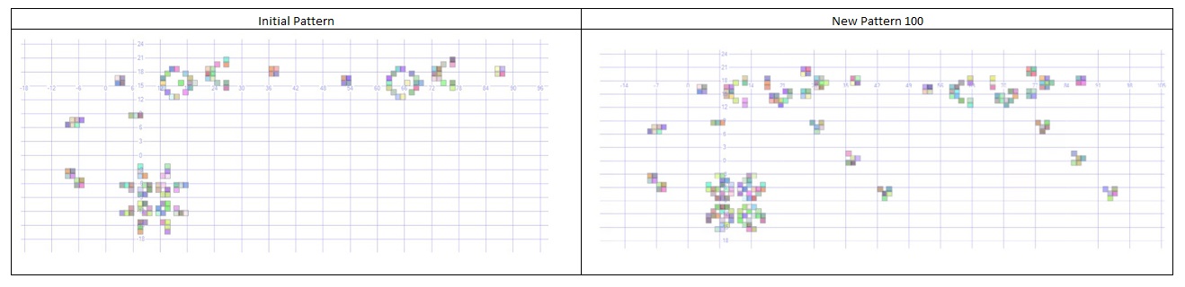
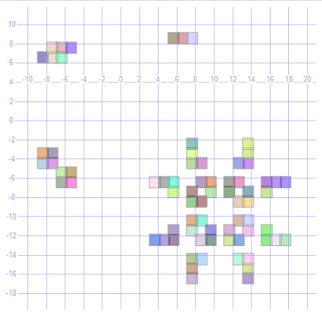
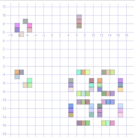
The screenshot below shows the initial patterns created at Stress Level 3.
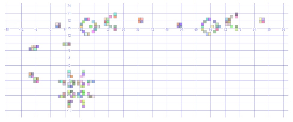
After 100 iterations, 6 new glider patterns have been created as shown below, 2 new gliders are created every 30th iteration which increases the CPU, IO and memory cost with each iteration.