

Introduction
With a new drive to move beyond the myopic traditional analytics to higher value driven Business Analytics (Analytics), one often requires more than one tool, development environment and analytic techniques to accomplish these endeavors.
The figure below indicates that, the higher the value you derive, the more difficult the analytics involved. This difficulty is known to be cumulative and comes from the fact that the higher the value the more tools you might need.
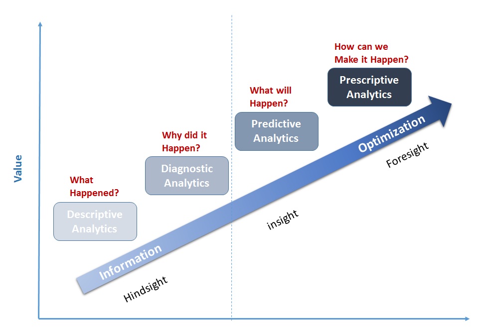
Figure1 : Value driven Analytics ( Source: Adapted from Gartner IT Glossary)
In this article we will look at developments in R and SQL Server that allows one to connect and work in both environments using T-SQL. Secondly, we will look at how data retrieved from SQL Server can be manipulated in-memory leveraging SQL-style R programming option and finally look at some of the ways one can take advantage of R's Exploratory data Analysis (EDA) and other advanced and more value driven analytics capabilities.
Why R and SQL Server?
In In a 2014 KDnuggets poll when asked, "What programming/statistics languages you used for analytics / data mining / data science work?" the top 3 languages were.
- R: 61%
- Python: 39%
- SQL: 37%
This means that for a lot of SQL folks, R is the statistics language of choice for analytics. Fortunately rsqlserver is a package in R that makes it is easy to work with R and SQL server databases using purely T-SQL for DDL and data retrieval queries. Benchmark tests shows it has 100X speed than ODBC options.
SQL and Data Munging
If you live in the real world very soon you find out that the clean cut data that comes with text books, courses and even those provided for data science competitions are not the reality. Sometimes it require more effort or "data munging" ( or "Data wrangling" as referred to in the Data Science Community) to get data to that form than the effort needed for all downstream analysis. There is evidence that Data scientists and data analysis experts spend well over 50% of the time collecting and preparing data before any exploration for useful insights begins. The good thing for SQL folks is, in the structured data world, SQL and RDBMs are still the most suited for this kind of work. Also, fortunately, in the un-structured data world, the many new SQL-based hadoop abstractions also means one is able to query semi-structured big data using SQL. Bottom line is, you have one leg up with SQL.
R
R is a free software programming language and software environment for statistical computing and graphics. But the capabilities of R are extended through user-created packages, which provides various specialized analytical techniques , graphical devices and utilities. Essentially, whatever data analysis problem you have there is likely an R package for it.
Even though most of the strategies reviewed in the article are SQL-based, the implementation assumes some familiarity with R and some concepts reviewed later, for those new to R you can learn more or download and installation from here.
RSQLSERVER
Rsqlserver is a DBI-compliant Sql Server driver based on the .NET Framework Data Provider for SQL Server (SqlClient). It is optimized to access a SQL Server directly without adding an OLE DB or Open Database Connectivity (ODBC) layer. For more on Rsqlserver and its installation visit <https://github.com/agstudy/rsqlserver> . It is important that you pay attention to the Prerequisites and package dependencies.
In this example, from R, we will connect to adventure works Database on a local SQL Server , create a complex view on the database and retrieve some data from the database using T-SQL .
First we load the libraries that are required to connect to the database.
library("rClr")
library("rsqlserver")
Next we create the connection string or the url and use it to connect as below.
url = "Server=localhost;Database=AdventureWorksDW2012;Trusted_Connection=True;"
conn = dbConnect('SqlServer', url=url)
CREATE VIEW [dbo].[vInternetSales]
AS
  WITH internetsales
       AS (SELECT pc.englishproductcategoryname,
                  COALESCE (p.modelname, p.englishproductname) AS Model,
                  c.customerkey,
                  s.salesterritorygroup                        AS Region,
                  CASE
                    WHEN Month(Getdate()) < Month(c.[birthdate]) THEN
                    Datediff(yy, c.[birthdate], Getdate()) - 1
                    WHEN Month(Getdate()) = Month(c.[birthdate])
                         AND Day(Getdate()) < Day(c.[birthdate]) THEN
                    Datediff(yy, c.[birthdate], Getdate()) - 1
                    ELSE Datediff(yy, c.[birthdate], Getdate())
                  END                                          AS Age,
                  CASE
                    WHEN c.[yearlyincome] < 40000 THEN 'Low'
                    WHEN c.[yearlyincome] > 60000 THEN 'High'
                    ELSE 'Moderate'
                  END                                          AS IncomeGroup,
                  d.calendaryear,
                  d.fiscalyear,
                  d.monthnumberofyear                          AS Month,
                  f.salesordernumber                           AS OrderNumber,
                  f.salesorderlinenumber                       AS LineNumber,
                  f.orderquantity                              AS Quantity,
                  cast(f.extendedamount as numeric)            AS Amount,
                  g.city,
                  g.stateprovincecode                          AS StateCode,
                  g.stateprovincename                          AS StateName,
                  g.countryregioncode                          AS CountryCode,
                  g.englishcountryregionname                   AS CountryName,
                  g.postalcode
           FROM   dbo.factinternetsales AS f
                  INNER JOIN dbo.dimdate AS d
                          ON f.orderdatekey = d.datekey
                  INNER JOIN dbo.dimproduct AS p
                          ON f.productkey = p.productkey
                  INNER JOIN dbo.dimproductsubcategory AS psc
                          ON p.productsubcategorykey = psc.productsubcategorykey
                  INNER JOIN dbo.dimproductcategory AS pc
                          ON psc.productcategorykey = pc.productcategorykey
                  INNER JOIN dbo.dimcustomer AS c
                          ON f.customerkey = c.customerkey
                  INNER JOIN dbo.dimgeography AS g
                          ON c.geographykey = g.geographykey
                  INNER JOIN dbo.dimsalesterritory AS s
                          ON g.salesterritorykey = s.salesterritorykey
),
   customersummary
       AS (SELECT customerkey,
                  region,
                  age,
                 IncomeGroup,
                  city,
                  statecode,
                  statename,
                  countrycode,
                  countryname,
                  postalcode,
                  sum(Quantity) as quantity,
                  cast(sum(Amount) as numeric) amount,
                  Sum(CASE [englishproductcategoryname]
                        WHEN 'Bikes' THEN 1
                        ELSE 0
                      END) AS Bikes
           FROM   internetsales AS InternetSales_1
           GROUP  BY customerkey,
                     region,
                     age,
                     city,
                     statecode,
                     statename,
                     countrycode,
                     countryname,
                     postalcode,
                     IncomeGroup)
  SELECT c.customerkey,
         c.geographykey,
         c.customeralternatekey,
         c.title,
         c.firstname,
         c.middlename,
         c.lastname,
         Cast(c.namestyle AS INT)            AS NameStyle,
         c.birthdate,
         c.maritalstatus,
         c.suffix,
         c.gender,
         c.emailaddress,
         Cast(c.yearlyincome AS INT)         AS YearlyIncome,
         Cast(c.totalchildren AS INT)        AS TotalChildren,
         Cast(c.numberchildrenathome AS INT) AS NumberChildrenAtHome,
         c.englisheducation,
         c.spanisheducation,
         c.frencheducation,
         c.englishoccupation,
         c.spanishoccupation,
         c.frenchoccupation,
         c.houseownerflag,
         Cast(c.numbercarsowned AS INT)      AS NumberCarsOwned,
         c.addressline1,
         c.addressline2,
         x.city,
         x.statecode,
         x.statename,
         x.countrycode,
         x.countryname,
         x.postalcode,
         c.phone,
         c.datefirstpurchase,
         c.commutedistance,
         x.region,
         x.age,
         x.IncomeGroup,
         cast(x.Amount as int) as Amount,
         x.Quantity,
         CASE x.[bikes]
           WHEN 0 THEN 0
           ELSE 1
         END                                 AS BikeBuyer
  FROM   dbo.dimcustomer AS c
         INNER JOIN customersummary AS x
                 ON c.customerkey = x.customerkey
Next, we pass the T-SQL query above as a string to the dbSendQuery() function using the connection we created above as shown below.
query = "
CREATE VIEW [dbo].[vInternetSales]
…………
"
dbSendQuery(conn, query)
Note that the dbSendQuery() function only synchronously submits and executes the SQL statement to the database engine. It does not extracts any records — to extract records with this command the query must return records after which the fetch()function must be used to retrieve the records as shown below.
query = "
SELECT [ModelRegion]
,[TimeIndex]
,[Quantity]
,cast ([Amount] as int) as Amount
,[CalendarYear]
,cast ([Month] as int) as Month
,[ReportingDate]
FROM [vTimeSeries] where [ModelRegion] like '%North America'
"
results = dbSendQuery(conn, query )
Sales_Dataframe = fetch(results, n = -1)
Whenever when you finish retrieving the records with the fetch() function make sure you invoke dbClearResult(). This clears the resultset from
Next we will use the dbGetQuery() to retrieve data given a database connection. This function submita, synchronously executes, and fetches data. Note that R holds the data retrieved with this function in-memory in what is called a dataframe. If you are not familiar with R you can think of a dataframe as an R version of a table.
In the following example data is retrieved from the vInternetSales view we created above.
InternetSales_Dataframe = dbGetQuery(conn, "Select * from vInternetSales")
From the logic above , InternetSales_Dataframe therefore becomes an in-memory dataframe (table) that can be further queried and used in various analysis in R as we will see later. You can check the structure and a few of the records in the dataframe as below.
#check the structure/definition of dataframe
str(InternetSales_Dataframe)
#top 10 records in the dataframe
head(InternetSales_Dataframe, 10)
#close(conn)
dbDisconnect(conn)
Value Driven Analysis using SQL-Style R syntax
At every stage of analytics there is always the potential to look at a subset or complex slice of your data regardless of what tool you choose. It is not easy to learn a new language so a good approach is to SQL-style syntax for data manipulation in languages when available. In this section I will show the most effective way (in my opinion) to continue working with your data from SQL Server in R using SQL-style syntax .
To continue working using SQL-Style R syntax, we will review R with respect to the SQL Logical query processing step below.
SQL Logical query processing step numbers
(4) SELECT <select_list>
(1) FROM Table
(2) WHERE <where_predicate>
(3) GROUP BY <group_by_specification>
(5) ORDER BY <order_by_list>;
The corresponding verbs (function Names) for R are as outlined in the table below. They are available in an R package called dplyr.
SQL | R |
FROM Table | data.frame() |
WHERE | filter() |
GROUP BY | group_by( ) |
SELECT | select() |
ORDER BY | arrange() |
Aggregate | summarise( ) |
Table 1
In R all aggregation are done in the summarise( ) function. Also, note that the verbs are all functions and can be used independent of each other unlike SQL key words. Therefore to combine them they must be chained together from left to right using the %>% symbol as shown in the example below.
SQL
select CountryName
,CountryCode
,StateCode
,Count(*) as Count
,TotYrIncome = sum(YearlyIncome)
,MaxYrIncome = max(YearlyIncome)
,MinYrIncome = min(YearlyIncome)
from [dbo].[vInternetSales]
where Gender ='F' and FirstName <>'NA' and LastName<>'NA'
group by StateCode, CountryCode, CountryName, (distinct FirstName), LastName
order by CountryName , StateCode
R
InternetSales_Dataframe %>%
filter( firstname!="NA" & lastname!="NA", gender=="F" ) %>%
group_by( statecode, countrycode, countryname) %>%
select (statecode, countrycode, countryname )%>%
summarise(
count = n()
,TotYrIncome = sum(YearlyIncome)
,MaxYrIncome = max(YearlyIncome)
,MinYrIncome = min(YearlyIncome)
)%>%
arrange( desc(countryname, statecode))
Pretty straight forward. Ironically the order of the R version follows the SQL Logical query processing step numbers outlined above.
So, what did I mean when I mentioned that the verbs could be used independently? See how all the R queries below return the same resultset as their SQL counterpart.
1. SQL :
select
maritalstatus, gender, YearlyIncome, TotalChildren, NumberCarsOwned, commutedistance, BikeBuyer
from InternetSales_Dataframe
where countrycode = 'US'
2. Chained - R:
InternetSales_Dataframe %>%
filter( countrycode =="US" ) %>%
select (maritalstatus, gender, YearlyIncome, TotalChildren, NumberCarsOwned, commutedistance, BikeBuyer)
3. Independent Functions - R:
US_Dataframe = filter(InternetSales_Dataframe, countrycode =="US" )
US_Dataframe = select (US_Dataframe,
maritalstatus, gender, YearlyIncome, TotalChildren, NumberCarsOwned, commutedistance, BikeBuyer)
4. True Functional style - R
US_Dataframe = select (
filter(InternetSales_Dataframe, countrycode =="US" )
,(maritalstatus, gender, YearlyIncome, TotalChildren, NumberCarsOwned, commutedistance, BikeBuyer)
)
When dealing with complicated queries especially with all the verbs, the unchained R versions (3 and 4) becomes cumbersome very quickly.
It must be noted that dplyr package can work with remote on-disk data stored in some databases. Currently dplyr supports the three most popular open source databases (sqlite, mysql and postgresql), and google's bigquery remotely on-disc database. But here we are going to use dplyr's to work with SQL-server data retrieved into a dataframe (in-memory) as above.
Statistical and Graphical analysis
As I mentioned earlier the strength of R lies in the availability of Packages for all sorts of tasks, more importantly for graphical and statistical analysis and modeling of data. In the following section I am going to show a few examples of how easy it is with the data we retrieved above. It most be noted that what I review here just scratches the surface of what R has to offer.
For instance let's see how easy to explore the data with R graphs. One such package is the ggplots package which can be loaded as below
library("ggplot2")
To check out how commuting distance affect bike sales by region we can plot the InternetSales_Dataframe data as below.
qplot(x = BikeBuyer, data = InternetSales_Dataframe,fill = factor(BikeBuyer) ,geom = "bar") + facet_grid(commutedistance ~ region)
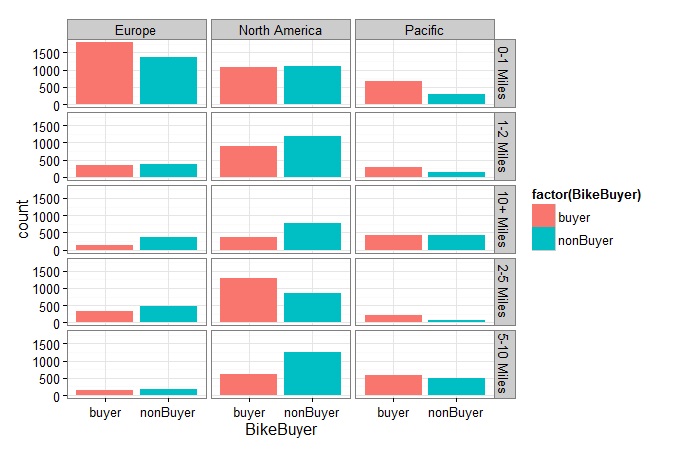
Figure 2: commuting distance and sales by region plot
From figure 2 above, it can be seen that in Europe and the Pacific customers who commute between 0-1 miles are more likely to buy bikes whiles in the US those who commute between 2-5 miles are more likely to buy bikes.
To check the sales trends of Specific bikes in North America we can plot the Sales_Dataframe data we retrieved earlier as below.
qplot(x = ReportingDate, y=Quantity, data = Sales_Dataframe, colour= factor(ModelRegion)
, group= factor(ModelRegion), geom = "line" )
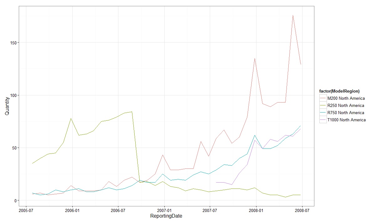
Figure 3: Sales trends of Specific Products in North America
It can be seen that the number of M200 and R750 models sold showed increasing trend with a seasonal pattern, while that of R200 model which also exhibited similar trend earlier experienced diminishing sales after dropping sharply around 2006-09.
Time Series Analysis and Forecasting
Another area R is strong is in Time series analysis, as I am going to demonstrate using the adventureworks sales data we used above. A lot of time series functions are available in the base installation.
As a simple exercise lets analyze sales of their best-selling M200 Model. A further examination of the M200 Model on figure above shows non-stationarity time series with an upward trend, a seasonal variation, and an increase of the seasonal oscillations over time in size. That means the series is not stationary. Let's try a natural log transformation of the original data after converting M200 Model data to a time series as below.
#get sales data for the M200 model
M200Sales_Dataframe <- filter(Sales_Dataframe, ModelRegion =="M200 North America")%>%
select (Quantity)
#convert to a monthly (frequency = 12) timeseries starting 0n 2005-07
M200Sales_TS <- ts(M200Sales_Dataframe ,frequency = 12, start = c(2005, 07))
#log transform original time series data
LogM200Sales_TS <- log(M200Sales_TS)
A plot of the log transformed data is shown below.
plot(LogM200Sales_TS)
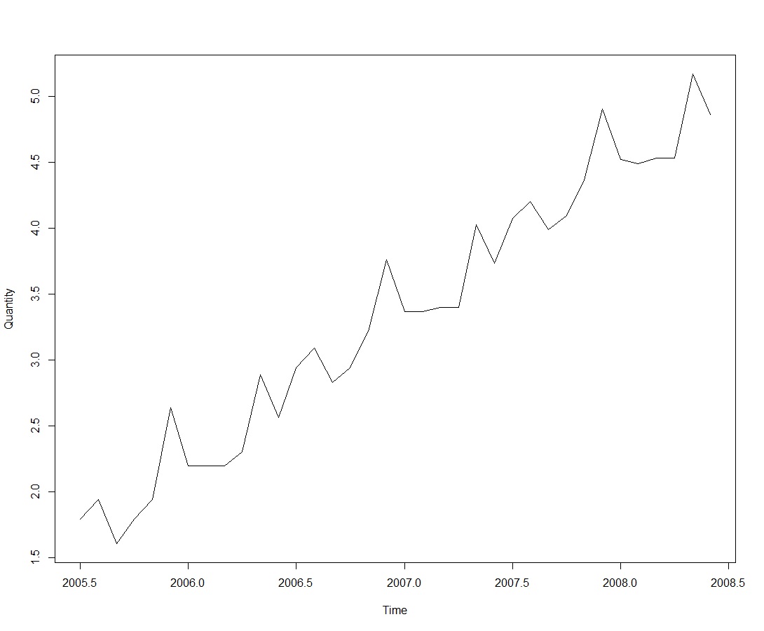
Figure 4: A plot of log of sales
From the plot of the log transformed data it can be seen that now the size of the seasonal and random fluctuations seem to be roughly constant over time. This suggests that the log-transformed time series may be described using an additive model.
Decomposing Seasonal Data
The various component patterns which includes the trend, seasonal and irregular components of the log-transformed time series can further be decomposed using the stl() function and plotted as shown below.
# Decompose a time series into seasonal, trend and irregular components using loess
LogM200Sales_DecomTS <- stl( LogM200Sales_TS[,1], s.window= "periodic")
#loess decomposition plot
plot(LogM200Sales_DecomTS, main= "Seasonal decomposition of log Sales using Loess")
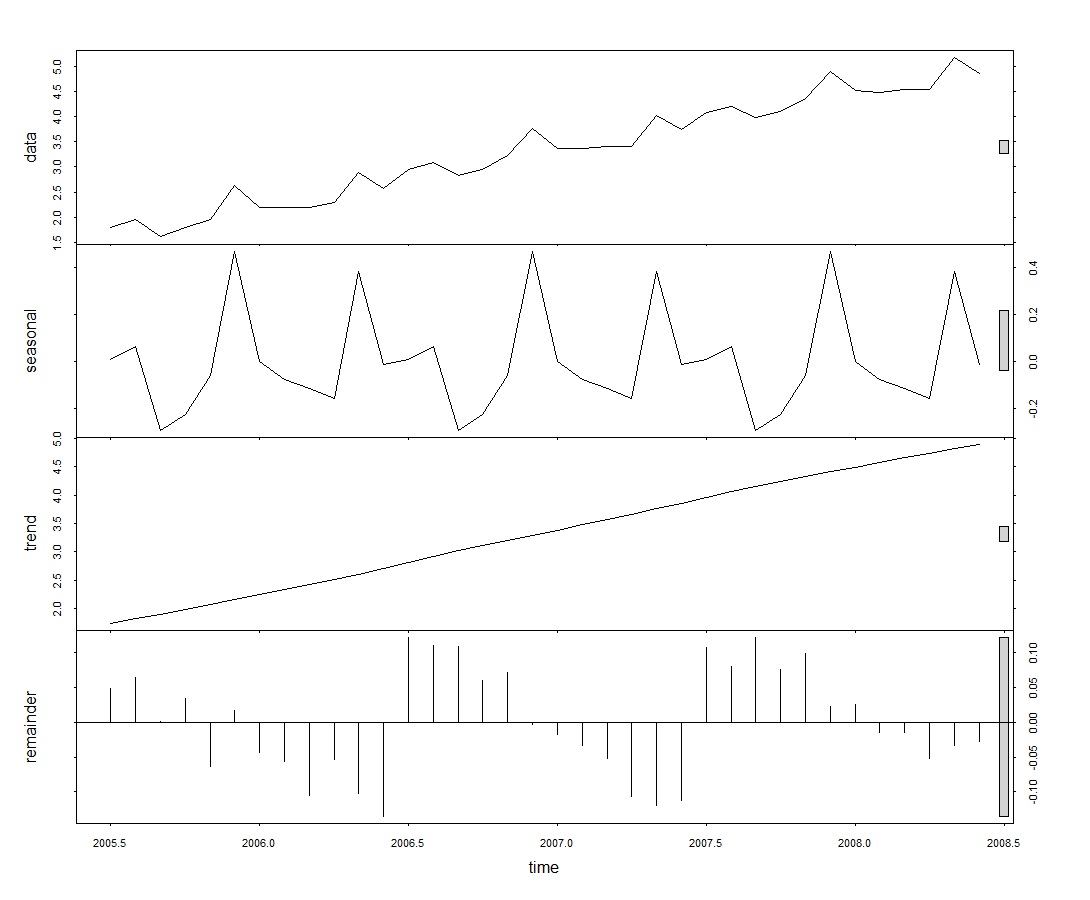
Figure 5: Plot of trend, seasonal and irregular components of the log-transformed time series.
The seasonal component now clearly show the seasonal peaks which occur before and after mid-year and the one larger seasonal peak that occurs just before the end of every year.
Exponential Models
A simple and very efficient modeling techniques that generates reliable forecasts is the exponential smoothing methods that generates weighted averages of past observations and decays the weights of the observations exponentially with time. The technique is implemented with a function called HoltWinters() in the R base installation as shown below.
fitM200Sales_TS <- HoltWinters(LogM200Sales_TS)
fittM200Sales_TS
The original log time series and the fitted values can be plotted as black and red lines respectively as below.
plot(fitM200Sales_TS)
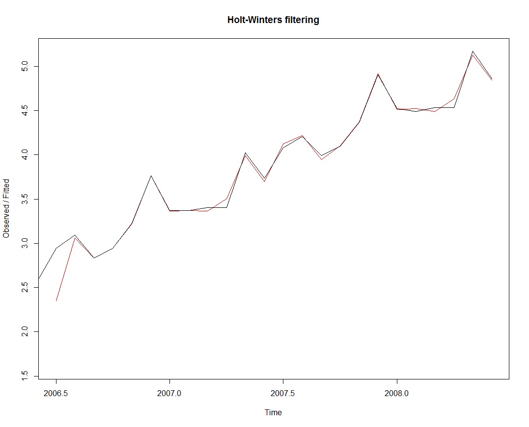
Figure 6: A plot of original and fitted values.
We see from the plot on figure 6 that the exponential method is very successful in predicting the seasonal peaks, which occur before and after mid-year and the one larger seasonal peak that occurs just before the end of every year.
To forecasts near future sales not included in the original time series we can use a package called forecast. For example, If we wanted to forecasts 12 months sales after the end of the time series, we load the forecast package and implement the forecasting on span>Holt-Winters fitted model as shown below.
library(forecast)
fcstM200Sales_TS<- forecast.HoltWinters(fitM200Sales_TS, h=12)
The forecasted values can plotted as below
plot.forecast(fcstM200Sales_TS)
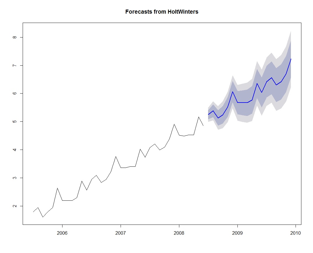
Figure 7: A plot of forecasted sales values
The forecast is shown as a blue line and the light blue and gray shaded areas show 80% and 95% prediction intervals, respectively.
ARIMA Models
Normally, a time series model could be improved upon by including correlation within prediction errors if there is evidence that there is any. If there is evidence, then more advanced techniques like ARIMA modeling processes that is also available in R could be used to improve the model. To check the model above, we can create a correlogram of the residuals using the sample autocorrelation function acf() as below.
acf(fcstM200Sales_TS_2$residuals, lag.max=20)
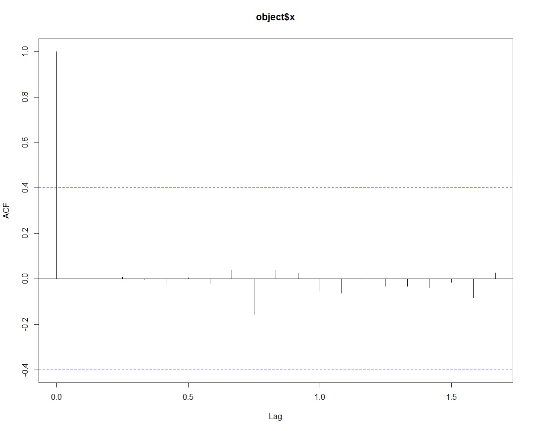
Figure 8: A correlogram plot of the residuals.
The plot shows that the autocorrelations of the residuals do not exceed the significance bounds for lags 1-20 which suggests that the model could likely not be improved by ARIMA models.
Predictive Modeling with Ensemble Methods
One area that R seems to stay ahead of the pack is in the area of new developments in machine learning methods, notably in the ensemble modeling techniques like Boosting and Random Forest. In many cases they performs better than the traditional classifiers like Decision Tree, Naïve Bayes and Logistic Regression especially where predictability is important than interpretability.
Ensemble methods are able to increase prediction accuracy by reducing variance through repeated fitting and averaging of training data.
For advanced R users with with predictive analytics experience, the result below shows how adaboost Boosting algorithm out-performs Naive Bayes using a subset of adventure works data useful for mail campaign analysis on customers who are likely or not likely to buy a bike. Running the query below generates the dataframe with the variables used in the modeling process.
DM_Dataframe <- InternetSales_Dataframe %>%
filter(countrycode =="US")%.%
select (maritalstatus, gender, YearlyIncome, TotalChildren,NumberChildrenAtHome,englisheducation, englishoccupation
,houseownerflag,NumberCarsOwned, countrycode, commutedistance,region, age, Amount, BikeBuyer)
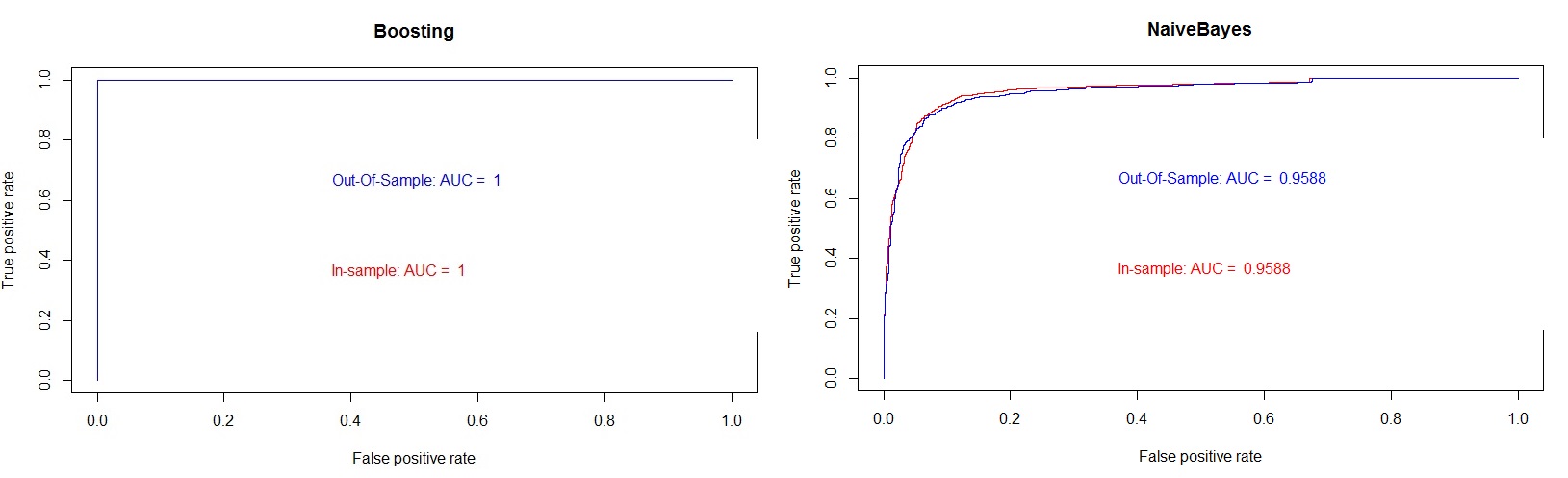
Figure 9: ROC plots showing in-sample and out-of-sample AUC values for Boosting and NaiveBayes.
The AUC of ROC metrics shown on the graphs from figure 9 above shows boosting model with better predictive power. The code used to fit the boosting model to the adventure works data is provided below. The code splits the data into a training and testing sets and further uses cross validation process to split the training dataset for in-sample and out-of-sample model validation.
library(ada)
set.seed(1234)
ind <- sample(2, nrow(DM_Dataframe), replace=TRUE, prob=c(0.7, 0.3))
train <- DM_Dataframe[ind==1,]
test <- DM_Dataframe[ind==2,]
model.fit <- ada(model.formula, data=train)
out.results.model.df<- data.frame()
In.results.model.df<- data.frame()
model.fit <- ada(model.formula, data=train)
#In-sample
in.model.predict<- predict(model.fit, train, type="prob" )
in.model.prediction <- prediction(in.model.predict[, 2], train$BikeBuyer)
in.model.auc <- attributes(performance(in.model.prediction, 'auc'))$y.values[[1]]
#out-of-sample
out.model.predict<- predict(model.fit, test, type="prob" )
out.model.prediction <- prediction(out.model.predict[, 2], test$BikeBuyer)
out.model.auc <- attributes(performance(out.model.prediction, 'auc'))$y.values[[1]]
outROCPerf <- performance(out.model.prediction , "tpr", "fpr")
inROCPerf <- performance(in.model.prediction , "tpr", "fpr")
plot(inROCPerf, main= "Boosting", col = "red")
legend(0.2,0.5,c(c(paste('In-sample: AUC = ', round(in.model.auc, digit=4))),"\n"), text.col= "red",
border="white",
cex=1.0,
box.col = "white")
plot(outROCPerf, col = "blue", add=TRUE)
legend(0.2,0.8,c(c(paste('Out-Of-Sample: AUC = ', round(in.model.auc, digit=4)),"\n"),text.col= "blue",
border="white",
cex=1.0,
box.col = "white")
Conclusion
SQL is a formidable language in value-driven analytics. It has solidify itself as the primary language for querying structured data. Also hadoop abstractions like spark, Hive etc. also means one is able to query semi-structured big data using SQL.
Often, more than one development environment is necessary for high-value driven analytics. By adopting SQL-style programming techniques in programming and statistics languages one can acquire the skillset needed to do a chunk of value-driven analytics. As shown here with few examples, SQL folks can utilize this strategy to take advantage of SQL Server and R environments benefiting from what both tools do best.