Power BI Desktop – the new self-service business intelligence tool from Microsoft – is already acquiring a reputation as being both impressively powerful and superbly easy to use. You can connect to multiple data sources and use them to create visually arresting dashboards that you can make available to users via the Microsoft cloud.
However nearly all BI entails showing how key metrics change over time. So in this article I want to provide an introduction to the vital set of functions that help you to use a time element when analyzing data. Power BI Desktop calls this feature “time intelligence” (even though it nearly always refers to is the use of date ranges). Applying this kind of temporal analysis can be a fundamental aspect of data presentation in business intelligence. After all, what enterprise does not need to know how this year’s figures compare to last year’s and what kind of progress is being made?
Time intelligence will always require a valid date table, which is one of the reasons why we will now spend a certain amount of time creating this core pillar of a successful data model. Then the date table has to be joined to the table containing the data that you want to compare over time on a date field. The good news is that once you have a valid date table, and have acquainted yourself with a handful of data and time functions in DAX, you can deliver some extremely impressive results. These kinds of calculations can cover (amongst other things)
- YearToDate, QuarterToDate, and MonthToDate calculations
- Comparisons with previous years, quarters, or months
- Rolling aggregations over a period of time, such as the sum for the last three months
- Comparison with a parallel period in time, such as the same month in the previous year
An introduction to time intelligence in Power BI Desktop will give you a taste of some of the DAX functions that you are likely to use when analyzing data over time. To begin with you will learn how to create a date table. Then you will take a look at a couple of the different types of calculation that you can create to analyze data over time once a date table has been added to your data model.
To get you started with Power BI Desktop this article comes with a small dataset that you can use as a starting point for the examples that are given below. This dataset consists of an Excel workbook containing the sample data and then a Power BI Desktop file that uses the Excel file as its source data. You will need to download these two files into the directory C:\PowerBiDesktopSamples on your local workstation.
Creating and Applying a Date Table
For time intelligence to work you will need a table that contains an uninterrupted range of dates that begins at least at the earliest date in your data, and that ends with a date at least equal to the final date in your data. In practice this will nearly always mean creating a date table that begins on the 1st of January of the earliest date in your data and that ends on the 31st of December of the last year for which you have data. Once you have your date table you can join it to one of the tables in your data model and then begin to exploit all the time-related analytical functions of Power BI Desktop.
The good news is that you can use Power BI Desktop itself to create a date table. It is also possible to import a contiguous range of dates from other applications such as Excel. As I would prefer you to come to appreciate the breadth and depth of Power BI in this article I will explain how to implement a data table directly in Power BI Desktop using some basic DAX.
Creating the Date Table
The first requirement before starting to apply time intelligence is to have a valid date table. The following few steps explain one way to create a date table using DAX.
1 - Open the Power BI Desktop file C:\PowerBiDesktopSamples\PowerBIDataModel.Pbix.
2 - Switch to Data View by clicking the middle icon on the left under the ribbon. You can see this icon in the image below.
3 - Activate the Modeling ribbon and click the New Table button. The expression Table = will appear in the Formula Bar.
4 - Replace the word Table with DateDimension.
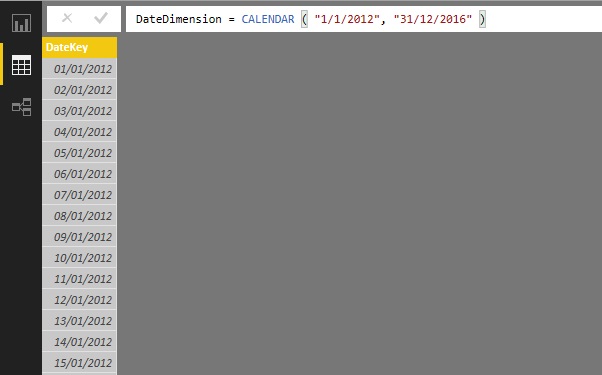
5 - Click to the right of the equals sign and enter the DAX function CALENDAR(.
6 - Enter "1/1/2012". This is the starting date for a table of dates. I am assuming here that your computer is configured for the UK or European date format. If this is not the case then enter the date as you would normally using your local date format
7 - Enter a comma.
8 - Enter "31/12/2016" (or the equivalent date format that represents the 31st of December 2016 in your local date format). This is the end date for a table of dates.
9 - Enter a right parenthesis. This corresponds to the left parenthesis of the Calendar() function. The formula Bar will display
DateDimension = CALENDAR( "1/1/2012", "31/12/2016" ).
10 - Press Enter or click the tick icon in the Formula Bar. Power BI Desktop will create a table containing a single column of dates from the 1st of January 2012 until the 31st of December 2016.
11 - In the Fields list, right-click on the Date field in the DateDimension table and select Rename. Rename the Date field to DateKey.The date table will look like the following figure.
12 - Click Anywhere inside the DateKey column.
13 - Click the New Column button in the Modeling ribbon. A new column will be added to the right of the existing columns.
14 - In the Formula bar replace Column = with
FullYear = YEAR([DateKey]).15 - Add 19 new columns containing the formulas explained in the Table below.
Column Title | Formula | Comments |
ShortYear | VALUE(Right(Year([DateKey]),2)) | Isolates the year as a two digit number |
MonthNumber | MONTH([DateKey]) | Isolates the number of the month in the year as one or two digits |
MonthNumberFull | FORMAT([DateKey], "MM") | Isolates the number of the month in the year as two digits with a leading zero for the first nine months |
MonthFull | FORMAT([DateKey], "MMMM") | Displays the full name of the month |
MonthAbbr | FORMAT([DateKey], "MMM") | Displays the name of the month as a three letter abbreviation |
WeekNumber | WEEKNUM([DateKey]) | Shows the number of the week in the year |
WeekNumberFull | FORMAT(Weeknum([DateKey]), "00") | Shows the number of the week in the year with a leading zero for the first nine weeks |
DayOfMonth | DAY([DateKey]) | Displays the number of the day of the month |
DayOfMonthFull | FORMAT(Day([DateKey]),"00") | Displays the number of the day of the month with a leading zero for the first nine days |
DayOfWeek | WEEKDAY([DateKey]) | Displays the number of the day of the week |
DayOfWeekFull | FORMAT([DateKey],"dddd") | Displays the name of the weekday |
DayOfWeekAbbr | FORMAT([DateKey],"ddd") | Displays the name of the weekday as a three letter abbreviation |
ISODate | [FullYear] & [MonthNumberFull] & [DayOfMonthFull] | Displays the date in the ISO (internationally recognised) format of YYYYMMDD |
FullDate | [DayOfMonth] & " " & [MonthFull] & " " & [FullYear] | Displays the full date with spaces |
QuarterFull | "Quarter " & ROUNDDOWN(MONTH([DateKey])/4,0)+1 | Displays the current quarter |
QuarterAbbr | "Qtr " &ROUNDDOWN(MONTH([DateKey])/4,0)+1 | Displays the current quarter as a three letter abbreviation plus the quarter number |
Quarter | "Q" &ROUNDDOWN(MONTH([DateKey])/4,0)+1 | Displays the current quarter in short form |
QuarterNumber | ROUNDDOWN(MONTH([DateKey])/4,0)+1 | Displays the number of the current quarter. This is essentially used as a sort by column |
QuarterAndYear | DateDimension[Quarter and Year] | Shows the quarter and the year |
MonthAndYearAbbr | DateDimension[MonthAbbr] & " " & [FullYear] | Shows the abbreviated month and year |
QuarterAndYearNumber | [FullYear] & [QuarterNumber] | Shows the year and quarter numbers. This is essentially used as a sort by column |
YearAndWeek | VALUE([FullYear] &[WeekNumberFull]) | Indicates the year and week. The VALUE() function ensures that the figure is considered as numeric by Power BI Desktop |
YearAndMonthNumber | Value(DateDimension[FullYear] & DateDimension[MonthNumberFull]) | A numeric value for the year and month. |
The first few columns of the DateDimension table should now look like the following figure.
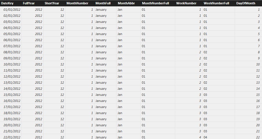
The point behind creating all these ways of expressing dates and parts of dates is that you can now use them in your tables, charts and gauges to aggregate and display data over time. Any record that has a date element can now be expressed visually not just as the date itself, but shown as-and aggregated as-years, quarters, months or weeks. The trick is to prepare all the time groupings that you are likely to need in the date table ready for your dashboards. However you do not need to worry if you find yourself needing an extra column or two further down the line as you can always add other columns that contain further date elements later.
Adding Sort By Columns to the Date Table
You now need to see how to sort a column using the data in another column to provide the sort order. This technique is essential when dealing with date tables, as you want to be sure that any visualizations that contain date elements appear in the right order. The classic example is months. As things stand, if you were to use the MonthFull or MonthAbbr columns in a chart or table then you would see the month names appearing on an axis or in a column in alphabetical order.
To avoid this you will have to add one final tweak to the date table and apply a Sort By column to certain of the date elements in other columns. Here is how:
1 - Click inside the column that you want to sort using the data from another column (MonthFull in this example).
2 - In the Modeling ribbon click on the Sort By button. A list of tha other columns in the table will appear – as shown in the following image.
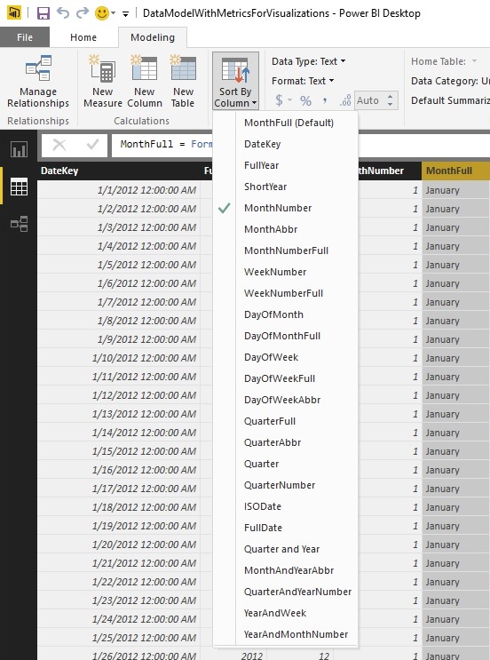
3 - Select the column that you want to sort by (MonthNumber in this example).
You will not see any immediate difference in the table of dates. However when you use any of the dates that you have tweaked in this way in a dashboard they will be sorted according to the order of the data in the Sort By column.
The table below gives you the required information to extend the data table that you have created so that all date elements are sorted correctly.
Column | Sort By Column |
MonthAbbr | MonthNumber |
DayOfWeekFull | DayOfWeek |
DayOfWeekAbbr | DayOfWeek |
Quarter And Year | QuarterAndYearNumber |
FullDate | DateKey |
MonthAndYearAbbr | YearAndMonthNumber |
MonthAndYear | YearAndMonthNumber |
Date Table Techniques
When using date tables to invoke time intelligence in DAX there are two fundamental principles that must always be applied.
- The date range must be continuous. That is there must not be any dates missing in the column that contains the list of calendar days in the table of dates.
- The date range must encompass all the dates that you will be using in other tables in the data model.
The first requirement is covered by the use of the Calendar() function to create a date table. The second can require that you discover the lower and upper date thresholds in one or more tables of dates. As this can be a little laborious (not to mention error-prone) it is probably easier to get DAX to find these dates for you and apply them to the Calendar() function.
Consequently, once you know where the lowest and highest dates are in your data model (even if they are in separate tables) you can use these dates as the lower and upper boundaries of the Calendar() function. In the case of the Brilliant British Cars (the company whose data we are analysing in the sample data set) data the formula could read
DateDimension = CALENDAR(MIN('Stock'[PurchaseDate]), MAX('Invoices'[InvoiceDate]))This formula shows that you can apply two functions that you have seen already -Min() and Max()-with date and datetime data types. They simply tell DAX to find the earliest and latest dates in a column.
Alternatively, and as a nod to best practice, you may prefer to ensure that the date dimension always covers entire years of dates. In this case the formula to create the table would be
DateDimension = CALENDAR(STARTOFYEAR(MIN('Stock'[PurchaseDate])), ENDOFYEAR(MAX('Invoices'[InvoiceDate])))This formula extends the DAX calculation using two functions that are extremely useful when creating date tables. These are
- StartOfYear() - This function deduces the first day of the year.
- EndOfYear() - This function deduces the last day of the year.
This formula also shows you that you can define a date range using different columns, or even different tables when you are specifying a date range. This is particularly useful when defining a date table.
Note The principal advantage of looking up the date boundaries like this is that they will update automatically as the source data changes. So if the Stock or Invoices tables are extended in the data source to contain further rows with dates outside the existing date range then the DateDimension table will also grow to encompass these new dates.
Creating a data table can be fun, but nonetheless takes a few minutes. So one tip I can give you is that you create a Power BI Desktop file that contains nothing but a date dimension table (using a manually defined start and end date just as you saw at the beginning of this example) with all the other columns added. You can then make copies of this "template" file and use them as the basis for any new data models that you create. This can include replacing the fixed threshold dates with references to the data in tables as mentioned previously.
Adding the Date Table to the Data Model
Now that you have a date table you can integrate it with your data model so that you can start to apply some of the time intelligence that DAX makes possible.
1 - Click on the Relationships View icon to display the tables in the data model.
2 - In the Home ribbon click the Manage Relationships button, The Manage Relationships dialog will appear.
3 - Click the New button. The Create Relationship dialog will appear.
4 - At the top of the dialog, select the DateDimension table from the popup list.
5 - Once the sample data from the DateDimension table is displayed, click inside the DateKey column to select it.
6 - Under the DateDimension table sample data, select the Invoices table from the popup list.
7 - Once the sample data from the Invoices table is displayed, click inside the InvoiceDate column to select it. The dialog will look like the figure below.
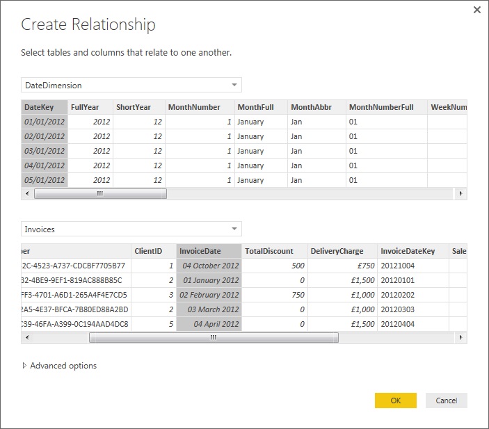
8 - Click OK. The relationship will appear in the Manage Relationships dialog.
9 - Click Close. The DateDimension table will appear in the data model joined to the Invoices table.
Note For time intelligence in Power BI Desktop to work correctly the fields used to join a date table and a data table must both be set to the date or datetime data type.
Applying Time Intelligence
Now that all the preparations have been completed it is (finally) time to see just how DAX can make your life easier when it comes to calculating metrics over time. This is possible only because you have a date table in place and it is connected to the requisite date field in the table that contains the data you want to aggregate. However with the foundations in place you can now start to deliver some really interesting and persuasive output.
YearToDate, QuarterToDate, and MonthToDate Calculations
To begin with, let's resolve a simple but frequent requirement: calculating month to date, quarter to date and year to date sales figures.
The three functions that you will see in this example are extremely similar. Consequently I will only explain the first one (a month to date calculation), and then will let you create the next two in a couple of copy, paste and tweak operations.
1 - In the Data View select the Invoices table and click New Measure.
2 - In the Formula Bar replace Measure with MonthSales.
3 - On the right of the equals sign enter (or type and select) TOTALMTD(. This will apply the month to date aggregation for a field.
4 - Enter (or type and select) SUM(. This specifies the actual aggregation that you want to apply.
5 - Select the field InvoiceLines[SalePrice] from the popup list of available fields.
6 - Enter a right parenthesis to end the Sum() function.
7 - Enter a comma.
8 - Type the first few characters of the date table (DateDimension in this example) and select the date key field (DateKey in this example).
9 - Enter a right parenthesis to end the Totalmtd() function. The formula should read
MonthSales = TOTALMTD(SUM(InvoiceLines[SalePrice]),DateDimension[DateKey])
10 - Press Enter or click the tick mark icon to complete the measure definition.
Now copy the formula that you just created and use it as the basis for two new measures. These will be quarterly sales to date and annual sales to date. The formulas are:
QuarterSales = TOTALQTD(SUM(InvoiceLines[SalePrice]),DateDimension[DateKey])
YearSales = TOTALYTD(SUM(InvoiceLines[SalePrice]),DateDimension[DateKey])
The three formulas that you have used are Totalmtd() for the Month to Date aggregation, Totalqtd() for the Quarter to Date aggregation, and Totalytd() for the Year to Date aggregation. All three functions take two parameters:
- The aggregate function to use (Sum() here—although it could be Average() or Count() or any other of the aggregate functions available in DAX), depending on the actual metric that you want to deliver and the table and column that is aggregated.
- The key field of the date table. Since the Invoices table is linked to the date table in the data model using the InvoiceDate field, DAX can apply the correct calculation if-and only if-you have added a date table to the data model and then specified the key field of the date table.
As you have created these measures I imagine that you would like to see them in action. The figure below shows the Quarter to date and Year to date sales for 2014 (along with the aggregated sales from the initial SalePrice column in the InvoiceLines table) in a simple Power BI Desktop table. To obtain this result you will have to drag the FullYear field from the DateDimension table onto the Page Level Filters area and then select only the check box for 2014. This will restrict the data to the year 2014.
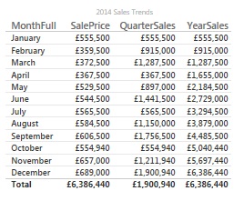
As you can see in this figure you have each month's sales figures along with the cumulative sales for each quarter to date (and restarting each quarter). The final column shows you the yearly sales total for each month to date. Also you will note that the months appear in calendar order as the MonthFull field has used the MonthNumber field as its Sort By column.
Conceptually the three functions that are outlined above (Totalmtd(), Totalqtd() and Totalytd() ) can be considered as DAX Calculate() functions that have been extended to deliver a specific result for a time frame. You can always calculate aggregations for a period to date using the Calculate() function if you want to. However as this "shorthand" version is so easy to use and so practical I see no reason to try anything more complicated when there is no real need.
Note In this example I suggest starting the process of adding a new measure with the Invoices table selected merely because this table seems a good place to store the metric. You can create the metric in virtually any table in practice-provided that you have a coherent data model to build on.
Pro Power BI Desktop
If you like what you read in this article and want to learn more about using Power BI Desktop, then please take a look at my book, Pro Power BI Desktop (Apress, May 2016).