
Microsoft has provided three Join operations for use in SQL Server. These operations are the Nested Loops, Hash Match and Merge Join. Each of these provides different benefits, and depending on the workload, one can be a better choice than the other two for a given query. The optimizer will choose the most efficient of these based on the conditions of the query and the underlying schema and indexes involved in the query. This article is the second of three in a series to explore these three Join Operations.
The first article in the series, on Nested Loops, can be found here.
Hash Match
The Hash Match represents the building of a hash table of computed hash values from each row in the input. From this MSDN article, this is the behavior of how that hash table is built. With a Hash match, you can expect to see the HASH:() and RESIDUAL:() predicates in an execution plan and potentially a probe row. This process works as follows:
- For any joins, use the first (top) input to build the hash table and the second (bottom) input to probe the hash table. Output matches (or non-matches) as dictated by the join type. If multiple joins use the same join column, these operations are grouped into a hash team.
- For the distinct or aggregate operators, use the input to build the hash table (removing duplicates and computing any aggregate expressions). When the hash table is built, scan the table and output all entries.
- For the union operator, use the first input to build the hash table (removing duplicates). Use the second input (which must have no duplicates) to probe the hash table, returning all rows that have no matches, then scan the hash table and return all entries.
In a Graphical Execution Plan, the Hash Match Operator looks like the following image.

When using the “set statistics profile” option, you will notice that the Hash Match will appear in your results, as shown in the following image.

In Action
How can we see the Hash Match in action? Let’s do a little setup to demonstrate the Hash Match. First let’s create some tables and then populate those tables with the following scripts.
  -- Create Tables
  SELECT TOP 25
          CustID = IDENTITY( INT,1,1 ),
          FirstName = 'George' + CHAR(ABS(CHECKSUM(NEWID())) % 26 + 65)
          + CHAR(ABS(CHECKSUM(NEWID())) % 26 + 65) ,
          LastName = 'Randcust' + CHAR(ABS(CHECKSUM(NEWID())) % 26 + 65)
          + CHAR(ABS(CHECKSUM(NEWID())) % 26 + 65) + CHAR(ABS(CHECKSUM(NEWID()))
                                                          % 26 + 65)
  INTO    dbo.Customer
  FROM    Master.dbo.SysColumns t1 ,
          Master.dbo.SysColumns t2
  GO
  SELECT TOP 1000000
          OrderID = IDENTITY( INT,1,1 ),
          CustID = ABS(CHECKSUM(NEWID())) % 25 + 1 ,
          OrderAmt = CAST(ABS(CHECKSUM(NEWID())) % 10000 / 100.0 AS MONEY) ,
          OrderDate = CAST(RAND(CHECKSUM(NEWID())) * 3653.0 + 36524.0 AS DATETIME)
  INTO    dbo.Orders
  FROM    Master.dbo.SysColumns t1 ,
          Master.dbo.SysColumns t2
  GO
  CREATE TABLE [dbo].[OrderDetail]
      (
        [OrderID] [int] NOT NULL ,
        [OrderDetailID] [int] NOT NULL ,
        [PartAmt] [money] NULL ,
        [PartID] [int] NULL
      );
  INSERT  INTO OrderDetail
          ( OrderID ,
            OrderDetailID ,
            PartAmt ,
            PartID
          )
          SELECT  OrderID ,
                  OrderDetailID = 1 ,
                  PartAmt = OrderAmt / 2 ,
                  PartID = ABS(CHECKSUM(NEWID())) % 1000 + 1
          FROM    Orders;
As you can see, I have created three tables for this simple example. None of these tables has an Index or a Primary Key at this point. Let’s run a query against two of these tables and see the results.
SELECT  O.OrderId ,
        OD.OrderDetailID ,
        O.OrderAmt ,
        OD.PartAmt ,
        OD.PartID ,
        O.OrderDate
FROM    Orders O
        INNER JOIN OrderDetail OD ON O.OrderID = OD.OrderID
The execution plan for this query looks like the following image:
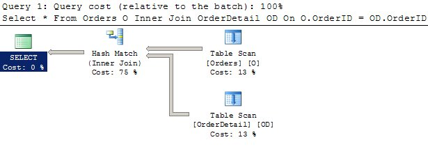
Here, we see that the query results in a Hash Match at this point. I could force a Nested Loops or Merge Join to occur if I were to use a query option, such as shown in the following queries.
SELECT  O.OrderId ,
        OD.OrderDetailID ,
        O.OrderAmt ,
        OD.PartAmt ,
        OD.PartID ,
        O.OrderDate
FROM    Orders O
        INNER JOIN OrderDetail OD ON O.OrderID = OD.OrderID
-- This is a hash match for this example
OPTION  ( LOOP JOIN )
 --force a loop join
SELECT  O.OrderId ,
        OD.OrderDetailID ,
        O.OrderAmt ,
        OD.PartAmt ,
        OD.PartID ,
        O.OrderDate
FROM    Orders O
        INNER JOIN OrderDetail OD ON O.OrderID = OD.OrderID
-- This is a hash match for this example
OPTION  ( MERGE JOIN ) --force a merge join
That is a simple enough change, and we have effectively been able to force a Hash Match into a different Join Operator. Is that really a wise thing to do? Keep in mind that we are querying a table that is without indexes. To see the impact of these Hints on this query, let’s examine some execution statistics.
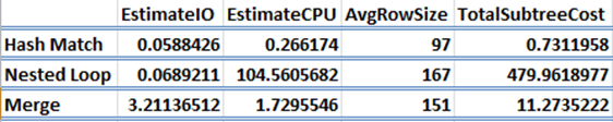
This illustrates the cost of this simple query using what the optimizer has determined to be the best Join Operator (Hash match) versus the effect of forcing a different Join Operator. The results are pretty telling on this query. It is no contest between the three operators that that Hash match is the best choice.
In the previous article about Nested Loops, I proceeded at this point to add indexes and so forth. For this article, I want to show what will happen by adding a third table to this query. After that, we will explore the effects of adding conditions to the predicate. Before proceeding, we will create a Clustered Index on each of the tables already created.
CREATE CLUSTERED INDEX CX_CustID ON Customer(CustID)
CREATE CLUSTERED INDEX CX_OrderDetailID ON OrderDetail(OrderId,OrderDetailID)
CREATE CLUSTERED INDEX CX_OrderID ON dbo.Orders(OrderID)
We will then execute the following query and retrieve the execution plan for it.
Select C.FirstName,C.LastName
            ,O.OrderId, OD.OrderDetailID, O.OrderAmt
            , OD.PartAmt, OD.PartID, O.OrderDate
      From Orders O
            Inner Join OrderDetail OD
                  On O.OrderID = OD.OrderID
            INNER JOIN Customer C
                  ON O.CustID = C.CustID;
Here is the complete execution plan:
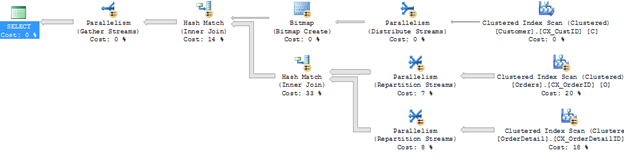
Notice that the query optimizer in this case continues to choose the Hash Match as the best Join Operator for this query. In this example, we see that the Hash Match is chosen for both Join Operators.
My next step is to filter the data. Finding a good predicate is essential when tuning a query. Depending on the predicate that is chosen, you could find a better or worse performing query. For the sake of this article, I have chosen two predicates to demonstrate and to compare to the use of the Join hints previously shown.
  SELECT  C.FirstName ,
          C.LastName ,
          O.OrderId ,
          OD.OrderDetailID ,
          O.OrderAmt ,
          OD.PartAmt ,
          OD.PartID ,
          O.OrderDate
  FROM    Orders O
          INNER JOIN OrderDetail OD ON O.OrderID = OD.OrderID
          INNER JOIN Customer C ON O.CustID = C.CustID
  WHERE   O.OrderID < 1000;
And second version of the query is:
SELECT  C.FirstName ,
        C.LastName ,
        O.OrderId ,
        OD.OrderDetailID ,
        O.OrderAmt ,
        OD.PartAmt ,
        OD.PartID ,
        O.OrderDate
FROM    Orders O
        INNER JOIN OrderDetail OD ON O.OrderID = OD.OrderID
        INNER JOIN Customer C ON O.CustID = C.CustID
WHERE   C.CustID < 25;
In this section I introduce a couple of terms that could use some clarification. Those terms are right-deep and left-deep. These terms are in reference to how a hash join is performed. When discussing left-deep vs. right-deep hashes, I find it useful to imagine a binary tree with a left leg and a right leg. A third term that I do not discuss is the bushy hash. Picture a bushy hash as a balanced binary tree where the left leg and the right leg are the same length. Then a right-deep and a left-deep can be easy to picture as either the right leg or the left leg being longer than the other leg. The length of that leg depends on the size of the inputs from the hash joins. The size from those inputs will impact when SQL server begins the probe phase. In a left-deep the probe all hash joins must complete before beginning the probe. With a right-deep hash, the probe can begin after the completion of the first hash build since that hash serves as an input to the next hash join.
The change in predicate is enough to sway performance of this query a considerable amount. The predicate of O.OrderID causes the Hash Match to be a right deep hash which happens to also eliminate the parallelism in this particular query. The predicate of C.CustID causes the query to utilize a left deep hash. What this means is that the O.OrderID causes the Hash Match to build the hash table on the two smaller tables (Customer and Orders) and then to probe against OrderDetails. This changes the memory requirements and changes the performance of the query. The following table helps to illustrate this performance shift.
PhysicalOp | LogicalOp | EstimateCPU | AvgRowSize | TotalSubtreeCost | Predicate | |
Hash Match | Inner Join | 0.05494589 | 58 | 0.127891 | Right Deep | O.OrderID |
Hash Match | Inner Join | 0.2354079 | 58 | 10.00208 | Left Deep | C.CustID |
Nested Loops | Inner Join | 0.008169726 | 58 | 0.3723499 | Nested Loops | O.OrderID |
Nested Loops | Inner Join | 0.1253654 | 58 | 29.79992 | Nested Loops | C.CustID |
Merge Join | Inner Join | 0.05638345 | 58 | 0.7106618 | Merge | O.OrderID |
Merge Join | Inner Join | 0.1253654 | 58 | 24.51446 | Merge | C.CustID |
For this particular query, the right deep version using the predicate of O.OrderID is the best plan to choose. That is, of course, if it meets the requirements. Also notice that for this example, the hash match query did outperform the Nested loops and the Merge Join operators within the respective predicates. It is also worth noting that continued tweaking of these predicates would eventually yield a less costly query that utilizes either the Merge Join or the Nested Loops operators.
Conclusion
The Hash Match join is a physical operator that the optimizer employs based on query conditions. The Hash Match can be seen in a graphical execution plan and can be employed with any join type yet does require an equijoin be present. The Hash Match Join is most likely to be the choice of the optimizer when one table has a large number of records.