

This is part 3 of a series on data mining. If you want to find part 1 and 2, you can find them here:
In the last chapter I talked about the decision tree algorithm. The decision tree is the first algorithm that we used to explain the behavior of the customers using data mining.
We found and predict some results using that algorithm, but sometimes there are algorithms that are better predictors of the future.
In this new article I will introduce a new algorithm.
The Microsoft Cluster Algorithm
The Microsoft cluster algorithm is a technique to group the object to study according to different patterns. It is different than the decision trees because the decision tree uses branches to classify the information. The Microsoft Cluster is a segmentation technique that divides the customer in different groups. This segments are not intuitive for humans.
For example, once the data mining algorithm detected that young man usually buy beer and diapers at the super market. It will group the customers according to different characteristics like the age, salary, number of cars, etc.

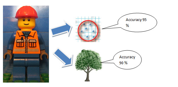
The figure displayed above shows a cluster. It is a segment of 7 customers grouped.
In this tutorial we are going to create a cluster algorithm that creates different groups of people according to their characteristics. The image below is a sample of how it groups:
You may ask yourself. When should I use decision tree and when to use cluster algorithm? There is a nice accuracy graph that the SQL Server Analysis Services (SSAS) uses to measure that. I will explain that graph in other article.
Now, let’s start working with the cluster algorithm and verify how it works.
Requirements
For this example, I am using the Adventureworks Multidimensional project and the AdventureworksDW Database. You can download the project and the database here:
http://msftdbprodsamples.codeplex.com/releases/view/55330
Getting started
Open the AdventureWorksDW Multidimensional project. If it is not processed, process it.
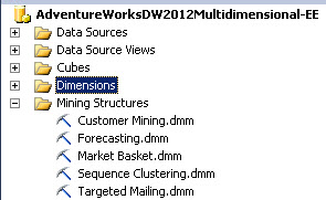
Open the Targeted Mailing dmm
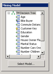
In this sample we are going to work with the targeted Mailing.dmm structure. Double click on it. Now click the Mining Models tab and you will get the image below.
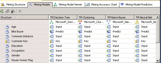
Mining models contains all the Models used to simulate the behavior of the customer. In this example we are using Decision Trees (explained in part 2 of these series). The decision trees and the cluster receive the same inputs of information. This information is a view named dbo. vTargetMail. This view contains customer information like the email, name, age, salary and so on.
In Data Mining Part 1 in the Data Mining Model Section you will find the steps to create a data mining structure. That structure can be used by other algorithms. In other words, once you have a structure created as an input for the model, you do not need to create it again for other algorithms.
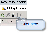
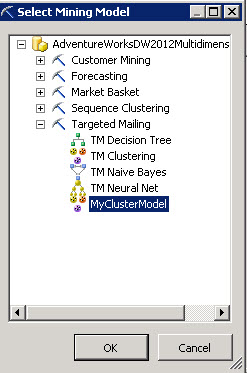
In this sample, the Cluster algorithm is already created. If it were not created, you only need to click the create a related mining model icon.
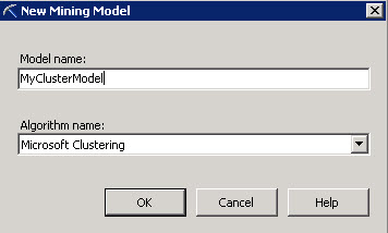
You only need to specify a name and choose the Algorithm name. In this case, choose Microsoft Clustering. Note that you do not need to specify input and prediction values because it was already done when you created your model in part 1 and 2 of the series.
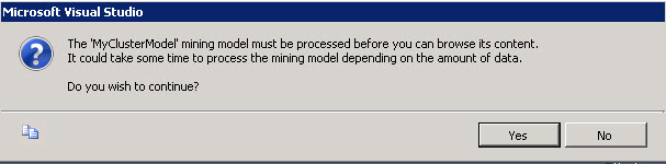
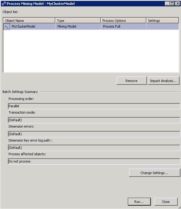
You will receive a message to reprocess the model, press Yes.
In the next Window press Run to process the Model.
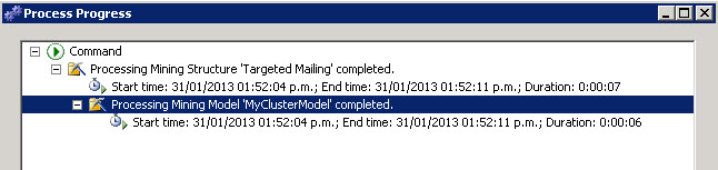
Once finished, the Mining structure will show the start time and the duration of the process.
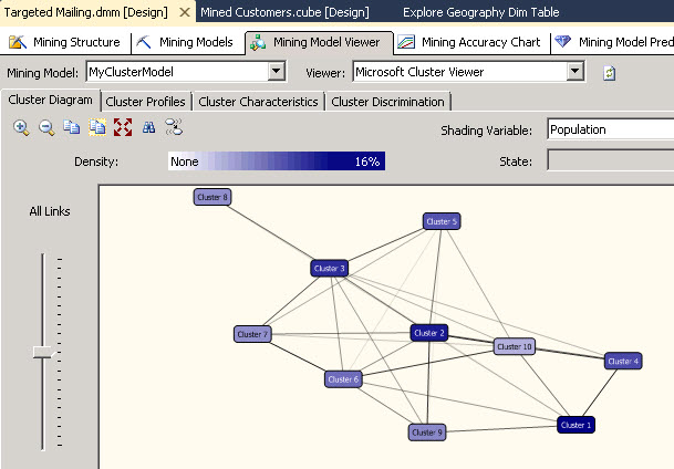
Go to the mining Model Viewer Tab and select the MyClusterModel just created to visualize the cluster algorithm. As you can see, it is an algorithm that creates different groups for all the customers. The groups are named cluster 1, cluster 2 and so on. The clusters creates groups of people based on their characteristis.
For example the cluster 1 contains people from Europe with a salary between 10000 and 35000 $us while the cluster 2 contains people from north america with a salary between 40000 and 1700000 $us. In the picture bellow you will find the different clusters created:
There are also different colors for the nodes. The darker colors are used for higher density clusters. In this case, the colors correspond to the Population. It is the shading variable. You can change the shading variable and the colors will change according to the value selected.
If you click in the cluster profiles, you will find the different variables and the population for each cluster. The total population is 18484. The cluster 1 is the most populated cluster and cluster 2 is the second 1. In other words, the clusters numbers are grouped according to the population.
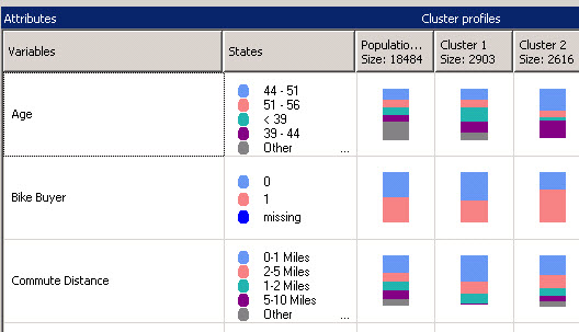
The variables show the customer’s characteristics like the age, salary and you can find the population with different colors for each characteristic. You can find interesting information here.
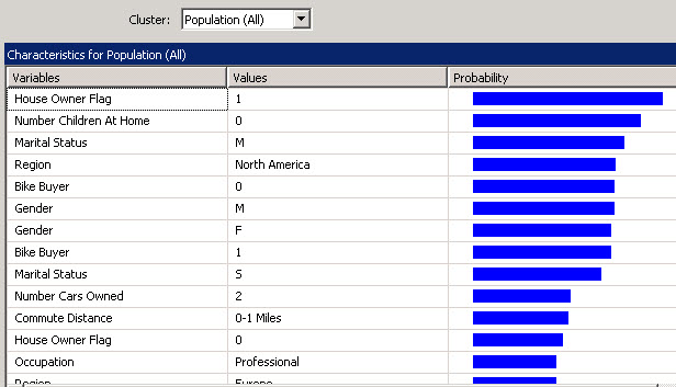
You can also click in the Cluster Characteristics Tab and Find the characteristics per cluster. In this example we are going to select the cluster 1.
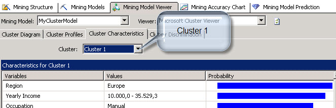
You will find here that the main characteristic of the cluster 1 is that the people are from Europe. That means that an important segment of people that buy bikes come are European. The second characteristic is the Yearly Income. We have the salary that is really important as well.
Note and compare the information from the decision tree (in chapter 2) and the cluster. The information provided is really different. We cannot say that the information from the decision tree is better than the cluster model. We can say that the information is complementary.
We also have the Cluster Discrimination tab. With this information you can visually find the differences between two clusters. For example, select Cluster 1 and Cluster 2.
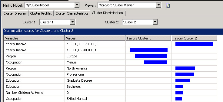
As you can see, the Yearly income is a big difference between these 2 clusters. The cluster 2 earns more money than the cluster 1. The same for the region, the cluster 2 do not necessarily live in Europe like the cluster 1. They are mainly Americans and earn more money.
As you can see you can work with different promotions for the different clusters with specific strategies.
Finally let’s predict the probability of the customer to buy a bike. The prediction section is the same as the decision trees. We can say that the Data Mining could be used like a black box to predict probabilities. In this example we are going to find the customer probability to buy a bike.
Click the Mining Model Prediction Tab. In the Mining Model, press the button Select Model.
In the select Mining Model select the model created at the beginning of this article (MyClusterModel).
I am not going to explain in detail the steps to select a Singleton Query because it was already explained in part 1 and go to the "predict the future section".
In part 1 we used the decision tree algorithm to predict the behavior of 1 customer with specific characteristics to buy a bike.
In this sample we are going to use repeat the same steps, but using the new cluster model created. In the steps 7 we are going to use different characteristics:
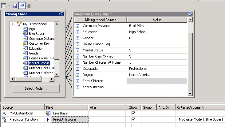
What we are doing here is asking to the cluster algorithm the probability of someone with a commute Distance of 5-10 miles with highschool education, Female, a house owner and single with 3 cars, one children professional and from north america to buy a house. We are using the cluster model created named MyClusterModel and we are using the PredictHistogram function a funcions that returns the probability from 0 to 1.
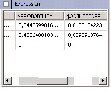
We will finally watch the results of the query:

In the results we will see that the probability to buy a bike is 0,544 (54 %) and the probability that the user will not buy is 0,45 (46 %).
Conclusion
In this chapter we used a new algorithm or method named Microsoft Cluster. The way that it organizes the information is different, but the input used is the same than the decision tree.
The output using the mining model prediction is the same, no matter the algorithm used. The results will be different according to the accuracy of the algorithm. We will talk about accuracy in latter chapters.
References
http://msdn.microsoft.com/en-us/library/ms174879.aspx
Images
http://userwww.sfsu.edu/art511_h/acmaster/Project1/project1.html
http://www.iglesiadedios.info/maranatha/2012/julio/eligiendo_c01.html