Introduction
The Cardinality Estimator (CE) is one of the main components of SQL Server Query Processor and its job is to estimate the number of rows that satisfies one or more predicates. CE answers the following questions:
- How many rows satisfy one single filter predicate? And how many satisfy multiple filter predicates?
- How many rows satisfy a join between two tables?
- How many distinct values are expected from a single column? And how many from a set of columns?
The Query Processor uses this information to find the most efficient query plan determining its shape and the components that fit better with the estimated row numbers calculated by CE. A wrong estimate could cause the Query Processor produce a poor strategy. These are some consequences of an underestimation or overestimation:
- A serial plan instead of a parallel plan or vice versa
- Poor join strategies
- Inefficient index selection and navigation strategies (seek vs scan)
- An inefficient quantity of reserved memory ending in spill in tempdb (underestimation case) or wasted memory (overestimation case)
Therefore, the CE is a very important component for SQL Server, but because of its nature, it is inherently inaccurate. It is built on statistics and assumptions about the uniformity of data distribution and independence between predicates.
The CE that SQL Server has been using since December 1998 (SQL Server 7 version), has been modified and adapted to all new features, but never rewritten. SQL Server 2012 still uses this “old” CE. The Microsoft development team has decided to redraw and rewrite a new CE for SQL Server 2014, changing many algorithms.
Obviously many bugs have been fixed and, on average, the estimates featured by the new CE are better than before and consequently the queries work better than before. There are though some cases where there is a risk of regression, due, for example, to bugs that hide other bugs in the old CE or new bugs in the new CE or simply due to different mathematical formulas applied.
In this article, we will see in detail some major differences between the two CEs and some cases in which one must be careful with using the new CE.
How to activate and deactivate the new CE
Having installed SQL Server 2014, to activate or deactivate the new CE, Microsoft suggests you change the database compatibility level. You can set it to 110 in order to leverage the previous CE, or set it to 120 for the new CE. Look at the following example with AdventureWorks2012 database:
--SQL Server 2012 compatibility level - Old Cardinality Estimator
ALTER DATABASE [AdventureWorks2012] SET COMPATIBILITY_LEVEL = 110
--SQL Server 2014 compatibility level - New Cardinality Estimator
ALTER DATABASE [AdventureWorks2012] SET COMPATIBILITY_LEVEL = 120
There is another unofficial way to do it and that is to use two Trace Flags:
- 2312 – to activate the new CE with a database set on 110 compatibility level
- 9481 – to activate the legacy CE with a database set on 120 compatibility level
You can also use these two flags directly in query using QUERYTRACEON option. See the following code as an example, where we use the old CE for a specific query, on a database set on 120 compatibility level:
USE AdventureWorks2012
GO
SELECT COUNT(*)
FROM Person.Person
OPTION (RECOMPILE, QUERYTRACEON 9481)
The advantage of this approach is that you can choose the best CE for each single query.
If you look at the execution plan, Actual or Estimated, you can see the leveraged CE in the property window of “SELECT” object. Value “70” means previous CE, “120” means new CE. The following image illustrates this.
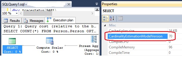
Properties window of “Select” component shows which CE has been used
Example with one predicate
With the following script we can create in tempdb dbo.Orders table with 1M rows:
USE tempdb
GO
IF OBJECT_ID('dbo.Orders') IS NOT NULL DROP TABLE dbo.Orders;
CREATE TABLE dbo.Orders(
  ID INT PRIMARY KEY IDENTITY(1,1)  NOT NULL,
  CustomerID INT NOT NULL,
  OrderDate DATETIME NOT NULL,
  TotalDue MONEY NOT NULL
 )
GO
-- Fill the table with 1M rows
DECLARE @DateFrom DATETIME = '20100101';
DECLARE @DateTo DATETIME = '20141231';
DECLARE @Rows INT = 1000000;
;WITH
CteNum (N) AS (Select 1
        UNION ALL
        SELECT N + 1
        FROM CteNum
        WHERE N < @Rows),
Ord (CustomerID, OrderDate, TotalDue) AS (
        SELECT ABS(BINARY_CHECKSUM(NEWID())) % 20000 AS CustomerID,
             (SELECT(@DateFrom +(ABS(BINARY_CHECKSUM(NEWID())) % CAST((@DateTo - @DateFrom)AS INT)))) AS OrderDate,
             ABS(BINARY_CHECKSUM(NEWID())) % 1000 AS TotalDue
        FROM CteNum)
INSERT INTO dbo.Orders
SELECT CustomerID, OrderDate, TotalDue
FROM Ord
OPTION (MAXRECURSION 0)
GO
--Create index on the OrderDate column
CREATE INDEX Idx_OrderDate ON dbo.Orders(OrderDate);
GO
Note. Because the values are randomly generated, your data distribution would be different from mine.
Let’s start now with a simple query on dbo.Orders table with one predicate that is a filter regarding the OrderDate field:
SELECT *
FROM dbo.Orders
WHERE OrderDate = '20141227'
OPTION (RECOMPILE, QUERYTRACEON 9481)
This query returns 593 rows and uses the old CE. If you look carefully at the execution plan putting the mouse pointer over the “SELECT” component, you will see that CE estimates 554.2 rows. If you execute the query again using the new CE, excluding the “QUERYTRACEON” option, you will see that the estimation remains the same.
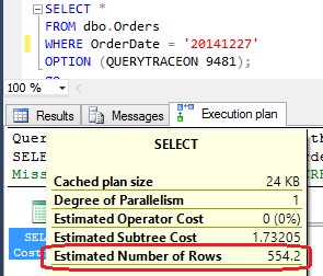
"Select" component tooltip shows Estimated Number of Rows
This value comes out from the statistic histogram of Idx_OrderDate index and it is AVG_RANGE_ROWS value of the histogram last step. This represents the average of rows expected for each value from 2014-12-24 to 2014-12-30.
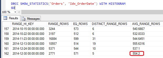
Idx_OrderDate Histogram
Until now both CEs have returned the same estimation, but we queried with up-to-date statistics. Let’s try to add 100000 rows with the following script; keep in mind that this number is less than 20% and for this reason it is too low to trigger an automatic statistics update.
DECLARE @DateFrom DATETIME = '20100101';
DECLARE @DateTo DATETIME = '20141231';
DECLARE @Rows INT = 100000;
;WITH
CteNum (N) AS (Select 1
        UNION ALL
        SELECT N + 1
        FROM CteNum
        WHERE N < @Rows),
Ord (CustomerID, OrderDate, TotalDue) AS (
        SELECT ABS(BINARY_CHECKSUM(NEWID())) % 20000 AS CustomerID,
             (SELECT(@DateFrom +(ABS(BINARY_CHECKSUM(NEWID())) % CAST((@DateTo - @DateFrom)AS INT)))) AS OrderDate,
             ABS(BINARY_CHECKSUM(NEWID())) % 1000 AS TotalDue
        FROM CteNum)
INSERT INTO dbo.Orders
SELECT CustomerID, OrderDate, TotalDue
FROM Ord
OPTION (MAXRECURSION 0)
GO
Now, if you query the statistic histogram again, you can observe than nothing has changed. If we carry out the query again, the previous CE continues to estimate 554.2, while the selected rows are now 658. The new CE estimates 609.62 rows and this is obviously better.
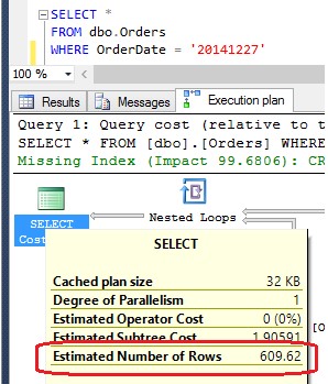
New CE estimation with not up-to-date statistics
Let’s now add some rows with DateOrder beyond the last value reported by the histogram and see how the behaviour of the two CEs changes. I would point out that this is a common scenario with ascending (or descending) keys. In fact, in a table with an ascending key, every record added after the last statistics update will have key value beyond the value reported in the last histogram step.
The following script adds 500 rows, all of them having OrderDate from 2015-01-01 to 2015-01-31.
DECLARE @DateFrom DATETIME = '20150101';
DECLARE @DateTo DATETIME = '20150131';
DECLARE @Rows INT = 500;
;WITH
CteNum (N) AS (Select 1
        UNION ALL
        SELECT N + 1
        FROM CteNum
        WHERE N < @Rows),
Ord (CustomerID, OrderDate, TotalDue) AS (
        SELECT ABS(BINARY_CHECKSUM(NEWID())) % 20000 AS CustomerID,
             (SELECT(@DateFrom +(ABS(BINARY_CHECKSUM(NEWID())) % CAST((@DateTo - @DateFrom)AS INT)))) AS OrderDate,
             ABS(BINARY_CHECKSUM(NEWID())) % 1000 AS TotalDue
        FROM CteNum)
INSERT INTO dbo.Orders
SELECT CustomerID, OrderDate, TotalDue
FROM Ord
OPTION (MAXRECURSION 0)
GO
The number of rows we have added is small and once again the statistics have not changed. If you run the query filtering by ‘2015-01-15’, the result, in my case, is 16 rows. Remember that we are generating rows with random values and your distribution of values may be different from mine.
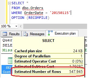
The previous CE estimates 1 row:
Old CE estimates 1 row
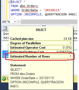
The new CE estimates 547.945 rows and in this case it is an overestimation, but it is in general better than 1.
In this case the new CE overestimates
Because the statistics are not up-to-date and the value we used as filter is not amongst the values known by the histogram, the new CE cannot use the above mentioned histogram. Therefore, it relies on the density vector and statistics header, in particular multiplying the number of rows (at the moment of the last statistic update) by the “All density” value of the density vector. See the picture below.
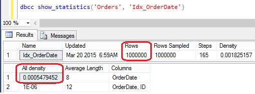
Statistics Header and Density Vector
Note. Until now we have used fixed values as filters. With variables, the CE cannot use the histogram and uses the Header and Density Vector again.
Multiple Predicates and the “Exponential Backoff” formula
The above examples use one predicate, but what happens with multiple filters? In the following example, we will use AdventureWorks2012 database and we will query against the Person.Address table. The following query has two predicates: the first filters for a specific value of StateProvinceId and the second for a range of values for PostalCode (Remove ", QUERYTRACEON 9481" in order to use the new CE):
SELECT *
FROM [Person].[Address]
WHERE StateProvinceID = 79
      AND
    PostalCode BETWEEN '98052' AND '98270'
OPTION (RECOMPILE, QUERYTRACEON 9481);
--Test for single predicates
SELECT *
FROM [Person].[Address]
WHERE StateProvinceID = 79
OPTION (RECOMPILE, QUERYTRACEON 9481);
SELECT *
FROM [Person].[Address]
WHERE PostalCode BETWEEN '98052' AND '98270'
OPTION (RECOMPILE, QUERYTRACEON 9481);
Using only the StateProvinceId filter, the result will be 2636 records and both CEs estimate exactly this number; using only the PostalCode filter the returned records will be 1121 and again both CEs estimate exactly this number. If we try using both filters, the selected rows will be 1120 because only one record with PostalCode between ‘98052’ and ‘98270’ has StateProvinceId different from 79.
Try running the query showing the execution plan and consider the Estimated Number of Rows for both CEs. The previous CE estimates 150.655 rows while the new CE estimates 410.956 rows and this is better because, it is not perfect, but it is nearer to the real number of selected records. But where does this difference come from?
The old CE assumes complete independence between the two predicates as if there were not any link between them; the new CE introduces new formulas presuming that there could eventually be some degree of dependence between the two predicates. The “Selectivity” of one predicate is defined as “Number of Selected Records” divided by “Number of all records of the table”. So, let S1 be the selectivity of the first predicate and S2 the selectivity of the second, the previous CE considers the selectivity of both predicates as S1 * S2. Multiplying the calculated selectivity by the number of all records of the table, we have the “Estimated Number of rows”.
The new CE applies a different formula called “Exponential back-off”, where S1 represents the selectivity of the most selective predicate, followed by the three most selective predicates:
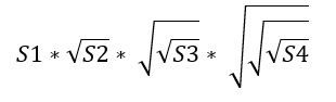
Exponential Back-Off Formula
Being the selectivity a number between 0 and 1, the square root function returns a bigger number than the given one, always less than 1 (or equal if the predicate returns all records of the table). In this way, the new CE calculates an Estimated Number of Rows which is higher than the old CE.
Going back to our example again, let’s see how the old and new CEs estimate the number of rows. Knowing 19614 is the total number of rows in Person.Adress table and having seen that both CEs estimate 2636 rows for StateProvinceId and 1121 rows for PostalCode, we can define:
S1 = 2636 / 19614
S2 = 1121 / 19614
Old CE estimate = S1 * S2 * 19614 = 150.655
New CE estimate = S1* SQRT(S2*19614) = 410.956
Obviously, the rightness of the result strictly depends on data distribution, but “Exponential back-off” formula guarantees a much more accurate estimate, because multiple predicates often have some degree of dependence.
Sometimes the old CE is better!
Sometimes you can end up in situations where the old CE works better than the new CE. The following script shows an example. Run it on AdventureWorks2012 database.
;WITH Cte
AS (SELECT CustomerId, OrderDate
    FROM (VALUES (29825, CAST('20050701' AS DATETIME)),
               (13006, CAST('20071121' AS DATETIME)),
               (19609, CAST('20071122' AS DATETIME)),
               (29842, CAST('20080601' AS DATETIME))) AS Wrk(CustomerId, OrderDate))
SELECT oh.OrderDate, OH.CustomerID, Cte.OrderDate
FROM [Sales].[SalesOrderHeader] oh
INNER JOIN Cte cte on oh.CustomerID = cte.CustomerId AND (oh.DueDate IS NULL OR oh.DueDate > cte.OrderDate)
OPTION (QUERYTRACEON 9481);
This query returns 16 rows. The previous CE estimates 14.0149 rows, and it is a very accurate estimation, while the new CE over estimates 24804.8 rows with a lot of wasted memory. In this case the guilty party is the “oh.DueDate > cte.OrderDate” join condition. It seems that the new CE doesn’t like it particularly.
Try yourself
There are a lot of examples we can use to understand in which cases the old CE works better than the new CE or vice-versa. Try yourself comparing the estimations and different execution plans that the two CEs generate in particular situations like:
- Varying the number of records of the tables referenced in query from a few dozens up to millions
- Joining two tables using null conditions or not equal conditions
- Using subqueries
- Working with updated and not updated statistics
- Varying the shape of the histogram related to a very selective or not selective index
- Filtering using mathematical functions and operators
Feel free to experiment other different situations.
Conclusion
SQL Server 2014 has introduced a new Cardinality Estimator based on different algorithms which generally works better than the old CE. However, there are cases where the old CE is more efficient and because of this it is recommended to do a lot of tests before using the new CE. There could be cases of regression.
You can leverage the new CE by putting the database Compatibility Level to 120 or leave it to 110 and continue using the old CE. In both cases, for particular queries, you can decide to use the other CE using QUERYTRACEON option with trace flags 2312 and 9481.