In our last episode, SQL Server was picking between index seeks and table scans, dancing along the tipping point to figure out which one would be more efficient for a query.

One of my favorite things about SQL Server is the sheer number of things it has to consider when building a query plan. It has to think about:

• What tables your query is trying to reference (which could be obfuscated by views, functions, and nesting)
• How many rows will come back from the tables that you’re filtering
• How many rows will then come back from other tables that you’re joining to
• What indexes are available on all of these tables
• Which indexes should be processed first
• How those indexes should be accessed (seeks or scans)
• How the data should be joined together between tables
• At what point in the process we’re going to need to do sorts
• How much memory each operator will need
• Whether it makes sense to throw multiple CPU cores at each operator

And it has to do all of this without looking at the data in your tables. Looking inside the data pages themselves would be cheating, and SQL Server’s not allowed to do that before the query starts executing. (This starts to change a little in SQL Server 2017 & beyond.)

To make these decisions,
SQL Server uses statistics.

Every index has a matching statistic with the same name, and each statistic is a single 8KB page of metadata that describes the contents of your indexes. Stats have been around (and been mostly the same) for forever, so this is one of the places where SQL Server’s documentation really shines: Books Online has a ton of information about statistics. You honestly don’t need to know most of that – but if you wanna make a living performance tuning, there’s a ton of great stuff in there.

For now, let’s keep it simple and just read our stat’s contents with DBCC SHOW_STATISTICS:

I don’t expect you to know or use that command often – if ever! – but knowing just a little bit about what’s happening here will start to shape how you think about query execution.

The first result set:

• Updated – the date/time this stat was last updated, either automatically or by your index maintenance jobs
• Rows – the number of rows in the object at the time the stats were updated
• Rows Sampled – just like a political pollster, as the population size grows, SQL Server resorts to sampling to get a rough idea of what the population looks like

The second result set shows the columns involved in the statistic – in our case, LastAccessDate, then Id. The first column is the main one that matters, though, because that’s where the histogram focuses, as the third result set shows.

Histograms sound complicated, but they’re really not so bad. I’ll walk you through the first two rows:

Each row is like a bucket.

The first row says, “The first LastAccessDate is August 1, 2008 at about midnight. There is exactly one row that equals this LastAccessDate.”

The second row says:

• Range_Hi_Key = 2008-11-27 – which means this bucket consists of all of the users who have a LastAccessDate > the prior bucket (2008-08-01), up to and including 2008-11-27.
• Eq_Rows = there is exactly 1 user with a LastAccessDate = 2008-11-27 09:02:52:947.
• Range_Rows = there are 1,222 other rows in this bucket.
• Distinct_Range_Rows = of those 1,222 rows, all of them have distinct LastAccessDates. That makes sense, since not everybody logs into StackOverflow.com at exactly the same time.
• Avg_Range_Rows = for any given LastAccessDate in this range, it only has 1 matching row. So if you filtered for WHERE LastAccessDate = ‘2008-10-15’, for example, SQL Server will estimate that 1 row will match.

That’s where your Estimated Number of Rows comes from.

When our query does this:

SQL Server pops open the histogram and scrolls down to the bottom (literally, he uses one of those old scroll mouse wheels) to review what he knows about the data as of the last time this stat was updated:

He scrolls down to the end and says, “Well, you’re looking for 2018-09-02 04:00. I don’t really have a bucket dedicated to just that, but I know that:

• Some of the rows in line 130 are going to match
• All of the rows in lines 131 and 132 are going to match

He cues up some Violent Femmes, adds them up, and comes up with an estimated number of rows. To see it, hover your mouse over the Index Seek and look at the bottom right:

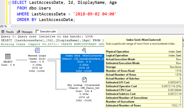
That’s a pretty doggone good estimate: he estimated 1,552 rows, and 1,576 rows actually came out. Good job, SQL Server. You get an A+ on your homework. Let’s pin this one on the fridge and take a look now at what your boy has done.

The easier of a time SQL Server has interpreting your query, the better job it can do. If your query tries to get all fancy and do things like functions or comparisons, then all bets are off, as we’ll see in the next episode.