One of the first successful programming languages was a relatively simple one named FORTRAN. This was short for “FORmula TRANSlator,” and it attempted to look as much like algebra as it could. The first version of this language had only two datatypes, integers and floating-point. You declared a variable by using it in the program; if the variable name began with the letters “I” thru “N”, then it was an integer, and otherwise it was a floating-point. Before you ask, yes, a typo could create a completely new variable on the fly. But don’t worry! There wasn’t much chance for confusion because variable names could only be six uppercase letters. Yes, I know it seems primitive, but please remember that our principle input device was a punch card while a pocket calendar today has more storage than all the computers that existed on earth back then.

It wasn’t until Algol 60 was invented that we saw the first modern block-structured programming language with something you would recognize as modern scoping rules. Serious programming language people often refer to Algol as being unique because it was better than most of the languages that came before and after it. This was the language that introduced begin-end blocks in programming and the concept of scoping.

Variables come into existence at the front of a begin-end block, persist during the execution of the code in that block, and then are deallocated when control exits that block. Most of you are probably used to using programming languages that follow this model. The syntactic sugar may change from keywords to curly brackets, but the storage model is still the same. There was a design flaw in the original Algol because we had not learned to think in scopes yet. While we did have if-then, if-then-else, begin-end and for-loop constructs, it wasn’t all we had! The language included a GOTO <label> statement that could change the flow of control to any spot in the program. This is what FORTRAN and all the other languages up until that time had. This was not a big problem when you had one and only one scope.

When the code jumps to the middle of a block, and exposes variables with the same name but a different scope, which one has priority? Perhaps a better question is that since we did not enter through the top of the block, does a local variable even exists since it was never allocated in the proper order? If they do exist, then what are their initial values? What are their values when you return to that block again from outside?

Later procedural programming languages got around these problems with the simple solution of getting rid of the GOTO statement. Every programmer should be required to read the classic article from the Communications of the ACM by Dykstra entitled The Go To Considered Harmful. This is what started the structured programming revolution in the 1970s.

The source of the term “structured” in structured programming was the ability to nest blocks inside each other. The goal is that each block would have one entry point and one exit point, and, ideally, it would perform one simple well-defined task. This allowed formal proofs of program correctness, optimization and other things as well as being a heck of a lot easier to maintain. The idea of scoping was carried from the Procedural Language Family into the declarative languages, like SQL. While we don’t have flow control, the structures in our language are also tiered or nested structures.

In SQL, you can nest queries inside each other via joins, set operations and other table level operations. This is actually a mathematical property called Orthogonality or Closure. In English, it is why operations done on numbers produce numbers, and you can add parentheses to mathematical expressions. Any place in which you can use a number, you can use a numeric expression. Anywhere in which you can use a table, you can use a table expression.

In SQL there is a hierarchy of schema objects in which the outermost level is the schema or database. The schema is made up of tables (which can be base or virtual tables) and other schema objects. Each of those tables is made up of a set of rows. These rows have no order, but all have the same structure, so it is a proper set. Each row is located by a key.

Each row is made up of columns, which can be real or virtual. The columns are scalar values drawn from a domain; a domain is set of values of one data type that has rules of its own. These rules include the type of scale upon which it is built and reasonable operations with it. Columns are located by their name, as qualified by the table in which they occur.

Transactions

Another vital concept is that of a unit of work, or a transaction. This means that when you do something in SQL, it either completes or it fails as a whole. But more than that, everything happens “all at once” in the transaction. The classic example of this is a simple update statement:

Please notice that this is a table-level transaction. It works on one and only one table. The columns X and Y will swap values because both assignments are made in parallel. Compare this to most procedural languages, which would execute the assignments left to right, record by record. The column X will get the value in column Y from the first assignment, and then column Y would get the same value put right back into it. This same pattern holds for computations in a SELECT list and everywhere else in the language. This is why when you update the table with an expression that has a timestamp in it, the timestamp has one initial value and is not incremented no matter how long it takes to physically write the rows to the schema.

You do not log in to a single table; you log on to the whole database and then use the DCL (Data Control Language) to find out which privileges you have on the constructs you can use. Once you have access to a table, the table is organized in rows, and then the rows are organized in columns. People often make the mistake of thinking that a table is “rows and columns” like a spreadsheet, but they are wrong. This concept is important because some statements work at the table level, some at the row level and some at the column level. When an operation is over, the table still has to be a table, and not full of assorted holes, mixed data types in a column, and so forth. For example, I can DROP TABLE <Tablename>; and get rid of the whole table. I can delete an entire row based on a predicate, DELETE FROM <Tablename> WHERE <search condition>;. But I cannot drop a few columns from a few rows in some odd tables. Likewise, I can’t just willy-nilly insert any old row in any old table.

Derived Tables

A derived table is a table expression embedded in a containing statement. It has to be placed inside parentheses, and it can optionally be given a correlation name and its columns can also optionally given names. The syntax is

If there is no (<derived column list>), then the derived table exposes the tables and their columns that created the derived table. Please notice that a simple table alias is a special case of a derived table. For some reason we don’t seem to think of an alias this way, but it is. Perhaps it’s because no SQL engine would actually be crazy enough to materialize an alias instead of using some kind of pointer structure.

The derived table will act as if it is materialized during the duration of the statement that uses it. Notice the phrase “act as if” in that last sentence. This phrase and the adjective “effectively” occur all over the ANSI/ISO SQL standards. To play safe, we also defined the execution of a query as being left to right, in the order written. This is important when we get to using infixed join operators, and in particular when we use the [LEFT | RIGHT | FULL] OUTER JOIN operators.

Set Operations

Likewise, the UNION [ALL], INTERSECT [ALL] and EXCEPT [ALL] operators are executed from left to right without precedence rules (this is not the way traditional set theory works). On top of these three traditional set operations, we also have OUTER UNION, DISTINCT and other options. Let me go ahead and say this: if you’ve done a good job of designing your schema, you probably will not find any use for “the fancy stuff” in your queries. In fact, the RIGHT OUTER JOIN is a rarity because we’re used to reading from left to right in programming languages based on the Latin alphabet.

The rules for the traditional set operations are that the tables involved must have the same structure. This is called “union compatible,” and it makes sense. The official definition of SQL will cast columns from different tables into the highest data type that is union compatible, but there is no obligation to keep the rows in the results in any particular order and nor do any of the columns in the result set have names unless you specifically give names to them.

In the very early days, various SQL products resolved the column names differently. Some took the names from the first table in the list of UNION-ed tables (SQL Server), some took the names in the last table, and some generated meaningless, long, ugly names.

The optimizer is free to re-arrange the clauses of a statement anyway that it wishes so long as the results are the same as the original statement. In fact, a really good optimizer can switch strategies during the execution of a single query when it runs into different parts of the data. The optimizer is where we get to show off how smart we are!

Once the query expression becomes a derived table with a correlation name, the internal structure is hidden. If no (<derived column list>) is given, then it inherits the column names from the component tables. Watch out; if the expression has two or more tables that have a common column name, you have to use <table name>. <column name> syntax to avoid ambiguity. This also happens to be a good programming practice.

In DB2, the optimizer can look at the mix of jobs, see if more than one session uses a view, and decide to materialize it and share it among sessions. Materialization is not an easy choice. If one statement uses a derived table, it might be better to integrate it into that statement like a text macro. But if many statements are using the same derived table, it might be better to materialize it once, and put the result in primary or secondary storage and share it. This is the same decision the SQL engine had to make with VIEWs. But the derived tables are not at the schema level where the optimizer can find them and keep statistics about them. It takes a pretty smart optimizer to select them for materialization. It might be better to put a derived table definition into a VIEW when it is reused often in systems where this functionality is supported.

Column Naming Rules

Derived tables should follow the ISO-11179 Standard naming rules. A table, base or virtual, is a table. The keyword AS is not required, but it is a good programming practice. If you do not provide names, then the SQL engine will attempt to do it for you. The table name will not be accessible to you since it will be a temporary internal reference in the schema information table. The SQL engine will use scoping rules to qualify the references in the statement — and what you said might not be what you meant. Likewise, columns in a derived table inherit their names from the defining table expression. But only if the defining table expression creates such names. As I already mentioned, the columns in a UNION [ALL], EXCEPT [ALL] or INTERSECT [ALL] statement have no names unless you use the AS clause. (SQL Server does use the names of the first query.)

When you have multiple copies of the same table expression in a statement, you need to tell them apart with different correlation names. For example, given a table of sports players, we want to query the team captain and team co-captain.

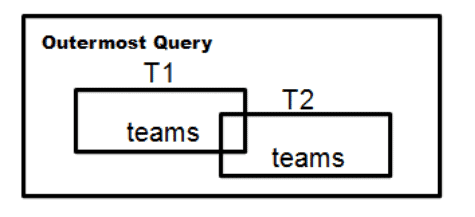
I have found that using a short table name abbreviation and a sequence of integers for correlation names works very well. This also illustrates another naming rule. The player’s last name is used in two different roles in this query, so we need to rename the column to the role name (if it stands by itself without qualification) or use the role name as a prefix (i.e., use boss_emp_id and worker_emp_id to qualify each employee’s role in this table).

Derived Tables

A derived table can be complete in itself without a scoping problem at all. For example, consider this query:

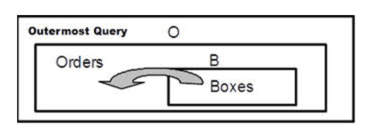
The derived table B has no outer references, and it can be retrieved immediately while another parallel processor works on the rest of the query. Another form of this kind of derived table is a simple scalar subquery:

The scalar subquery is computed; the one row, one column result table is converted into a unique scalar value, and the WHERE clause is tested. If the scalar subquery returns an empty result set, it is converted into a NULL. Watch out for that last case, since NULLs have a data type in SQL, and in some weird situations you can get casting errors.

When a table expression references correlation names in which they are contained, you have to be careful. The rules are not that much different from any block-structured programming language. You work your way from the inside out.

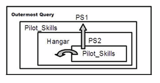
This is easier to explain with a classic relational division example. We have a table of pilots and the planes they can fly (dividend); we have a table of planes in the hangar (divisor); we want the names of the pilots who can fly every plane (quotient) in the hangar. This is Chris Date’s version of Relational Division; the idea is that a divisor table is used to partition a dividend table and produce a quotient or results table. The quotient table is made up of those values of one column for which a second column had all of the values in the divisor.

The quickest way to explain what is happening in this query is to imagine a World War II movie where a cocky pilot has just walked into the hangar, looked over the fleet, and announced, “There ain’t no plane in this hangar that I can’t fly!” This is terrible English but sound logic.

Notice that PilotSkills appears twice in the query, as PS1 and as PS2. We have a local copy of PilotSkills as PS2 and outer references to tables H and PS1. We find that H is a copy of the Hangar table one level above us. We find that PS1 is a copy of the PilotSkills table two levels above us.

If we had written WHERE pilot_name = PS2.pilot_name in the innermost SELECT, the scoping rules would have looked for a local reference first and found it. The search condition would be the equivalent of WHERE PS2.pilot_name = PS2.pilot_name, which is always TRUE since we cannot have a NULL pilot name. Oops, not what we meant!

It is a good idea to always qualify the column references with a correlation name. Hangar did not actually need a correlation name since it appears only once in the statement, but do it anyway. It makes the code a little easier to understand for the people that have to maintain it — consistent style is always good. It protects your code from changes in the tables. Imagine several levels of nesting in which an intermediate table gets a column that had previously been an outer reference.

Exposed Table Names

The nesting in SQL has the concept of an “exposed name” within a level. An exposed name is a table name that is not followed by a correlation name, or a view name that is not followed by a correlation name. The exposed names must be unique.

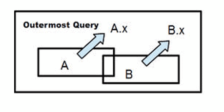
Here are some examples to demonstrate scoping rules.

Tables A and B can be referenced in the outer WHERE clause. These are both exposed names, but this won’t work in SQL Server which requires you to name a derived table.

You can scope them into a new table, X like:

But only Table X can be referenced in the outer WHERE clause. The correlation name X is now an exposed name.

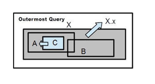
Table C is not exposed to any other SELECT statement.

Common Table Expressions

ANSI/ISO Standard SQL-99 added the Common Table Expression or CTE. It is also a query expression that is given a name, just like a derived table. The difference is that they appear before the SELECT clause in which they are used. This is the same as factoring out a common subexpression in algebra! They are just a very useful bit of syntactic sugar. The only thing to remember is that each CTE is exposed in the order they appear in the WITH clause. That means the n-th CTE in the list can reference the first thru (n-1)-th CTEs, but it has to reference them in the order written.

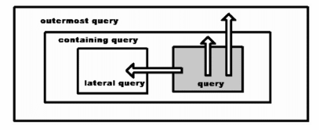
LATERAL Tables

If you have worked with blocked structured procedural languages, you will understand the concept of a “Forward Reference” in many of them. The idea is that you cannot use something before it is created in the module unless you signal the compiler. The most common example is a set of co-routines in which Routine A calls Routine B, then Routine B calls Routine A and so forth. If Routine A is declared first, then calls to B must an additional declaration that tells the compiler Routine B will be declared later in the module. T-SQL does not have this feature yet, but you can use APPLY to get some of the same results. This might be easier to demonstrate than to explain. The following example runs, but it returns the overall average salary and employee count, not the values for each department:

Notice that the Departments table appears as D1 and D2 at two levels – D1 is at level one and D2 is a level three.

The following example is not valid because the reference to D.dept_nbr in the WHERE clause of the nested table expression references the Personnel table via P.dept_nbr that is in the same FROM clause.

To make the query valid, we need to add a LATERAL clause in front of the subquery. Notice the order of Personnel and Departments. This exposes the department number so that a join can be done with it in the derived table labelled E.

 

To do the same thing in T-SQL, use CROSS APPLY.

Programming Tips

Let me finish with some heuristics.

1. Use aliases that tell the guy maintaining this code what tables are referenced. Do not simply use A, B, C, etc., as names. This comes from the 1950s when files were referenced by the name of the tape drive that held them.

2. Always “Pretty print” the SQL so that the indentation tells the reader what the query structure is. This is a simple task for any of many tools.

3. Never use SELECT * in production code; it will eventually bite you when a table changes. You have a text editor, and it is easy to cut & paste a list of column names.

4. When you have three or more levels of nesting, think about a CTE. The code will be more readable.

5. When you have two or more references to a query expression think about a CTE or a VIEW if the expression is used in several statements. The code will be more readable, but in many SQL systems, it will also help the optimizer make a decision about materialization.