

In the previous post, I showed how you can get full listings of your execution plan costs. Knowing what the values you’re dealing with for the estimated costs on your execution plans can help you determine what the Cost Threshold on your system should be. However, we don’t want to just take the average and use that. You need to understand the data you’re looking at. Let’s explore this just a little using R.
Mean, Median, Range and Standard Deviation
I’ve used the queries in the previous blog post to generate a full listing of costs for my plans. With that, I can start to query the information. Here’s how I could use R to begin to explore the data:
library("RODBC", lib.loc="~/R/win-library/3.2")
query <- "SELECT * FROM dbo.QueryCost;"
dbhandle <-
  odbcDriverConnect(
    'driver={SQL Server};server=WIN-3SRG45GBF97\\dojo;database=AdventureWorks2014;trusted_connection=true'
  )
data <- sqlQuery(dbhandle,query)
##data
mean(data$EstimatedCost)
median(sort(data$EstimatedCost))
maxcost = max(data$EstimatedCost)
mincost = min(data$EstimatedCost)
costrange = maxcost - mincost
costrange
sd(data$EstimatedCost)
The mean function is going to get me my average value, which, in this case, is 0.8755985. If I just accept the average as a starting point for determining my Cost Threshold for Parallelism, I guess I can just leave it at the default value of 5 and feel quite comfortable. This is further supported by the median value of .0544886 from my data. However, let’s check out the costrange value. Knowing an average, a mean, or even a median (literally, the middle number of the set), doesn’t give you an indication of just how distributed the data is. My costrange, the max minus the min, comes out to 165.567. In other words, there is a pretty wide variation on costs and suddenly, I’m less convinced that I know what my Cost Threshold should be.
The next value that matters is the Standard Deviation. This gives you an idea of how distributed your data is. I’m not going to get into explaining the math behind it. My standard deviation value is 8.301819. With this, I know that a pretty healthy chunk of all my values are less than a cost estimated value of 8, since a single standard deviation would be 8.301819 on top of my average value of .8755985.
With this knowledge, I can start to make informed choices. I’m not relying simply on an average. I can begin to think through the process using statistics.
Just to help out with the thought process, let’s plot the values too.
Histogram
My first thought for any kind of data is statistics, so let’s see what a histogram would look like. This is really easy to do using R:
hist(data$EstimatedCost)
The output looks like this:
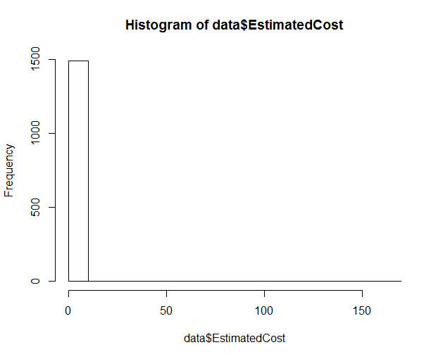
Clearly, this doesn’t give me enough to work on. Most of my data, nearly 1500 distinct values, is at one end of the distribution, and all the rest is elsewhere. I can’t use this to judge any kind of decision around my Cost Threshold.
Scatter Plot
The histogram isn’t telling me enough, so let’s try throwing the data into a Scatter plot. Again, this is silly easy in R:
plot(data$EstimatedCost)
The output is a lot more useful:
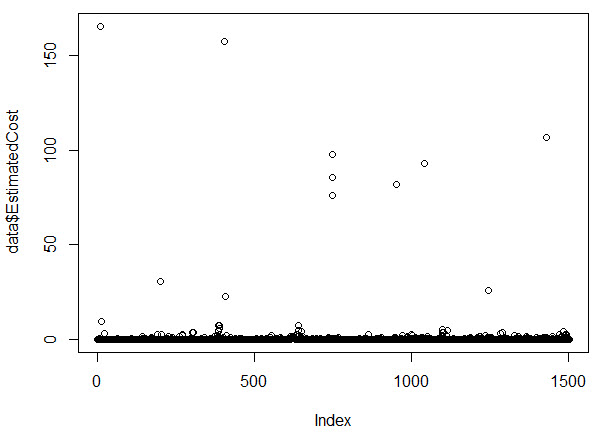
Now I can begin to visually see what the standard deviation value was telling me. The vast majority of my costs are well below two standard deviations, or approximately 16. However, let’s clean up the data just a little bit and make this as clear as we can.
Density Plus Values
Instead of just plotting the values, let’s get the density, or more precisely, a kernel density estimation, basically a smooth graph of the distribution of the data, and plot that:
plot(density(data$EstimatedCost))
rug(data$EstimatedCost,col='red')
I went ahead and added the values down below so that you can see how the distribution goes as well as showing the smooth curve:
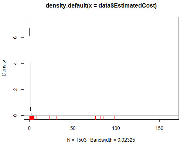
That one pretty much tells the tale. The vast majority of the values are clumped up at one end, along with a scattering of cost estimates above the value of 5, but not by huge margins.
Conclusion
With the Standard Deviation in hand, and a quick rule of thumb that says 68% of all values are going to be within two standard deviations of the data set, I can determine that a value of 16 on my Cost Threshold for Parallelism is going to cover most cases, and will ensure that only a small percentage of queries go parallel on my system, but that those which do go parallel are actually costly queries, not some that just fall outside the default value of 5.
I’ve made a couple of assumptions that are not completely held up by the data. Using the two, or even three, standard deviations to cover just enough of the data isn’t actually supported in this case because I don’t have a normal distribution of data. In fact, the distribution here is quite heavily skewed to one end of the chart. There’s also no data on the frequency of these calls. You may want to add that into your plans for setting your Cost Threshold.
However, using the math that I can quickly take advantage of, and the ability to plot out the data, I can, with a much higher degree of confidence, make choices on how I want my Cost Threshold for Parallelism to be set on my servers. From there, I measure the affects of my choices and adjust as necessary.
The post Determining the Cost Threshold for Parallelism appeared first on Grant Fritchey.
![]()
