Nonclustered indexes overview

Indexes are a necessity for most tables of any substantial size. When indexes are strategically and purposefully created, they can provide efficient and precise data access by allowing the query optimizer to find the best and shortest route to a desired result set. This is accomplished by using a B-tree method of quickly locating the index’s pointer to the actual data values that the query is requesting.

The benefits of traditional indexes, however, come at a cost. Nonclustered indexes are created as structures that are distinct from the data that they organize – essentially, a nonclustered index is a copy (of sorts) of the table, storing data for every row of the table. Therefore, the more records in a table, the larger the index must be – increasing the overall data storage cost for the table. Also, index maintenance times are increased as each new index is added. Indexes must be reorganized at certain intervals to maintain accuracy. An index becomes inaccurate as data is changed – insert, update, delete, and merge operations all create a maintenance requirement.

Traditional nonclustered indexes target all data in a column – including NULL values – even if certain values are never searched for.

In light of all this, it’s not surprising that Microsoft has provided a special type of index that optimizes and enhances traditional nonclustered indexes: filtered indexes. Let’s look at what they are and how they are used.

Filtered nonclustered indexes

Filtered indexes for SQL Server were introduced in SQL Server 2008. Put simply, filtered indexes are nonclustered indexes that have the addition of a WHERE clause. Although the WHERE clause in a filtered index allows only simple predicates, it provides notable improvements over a traditional nonclustered index. This allows the index to target specific data values – only records with certain values will be added to the index – resulting in a much smaller, more accurate, and more efficient index.

The basic syntax for creating a filtered index is:

Let’s set up a basic filtered index on the Sales.SalesOrderDetail table in the AdventureWorks2012 sample database. Since it’s the largest table in the database (more than 121,000 records), it should give us the best opportunity to see the benefits of a filtered index. The query we will be using will look like this, initially:

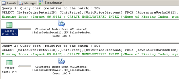
If we look at the current execution plan for this query, we see that there are no existing indexes that could be used for an index seek to locate the matching records efficiently, and that a clustered index scan was performed instead. An index seek operation happens when the query engine is able to use an appropriate index to find the exact location of the requested data, using the b-tree method. An index scan operation happens when every row of an index must be examined in order to find values in columns that the index does not cover. We see that for our query, the clustered index was scanned to locate rows that match the given criteria for the UnitPrice column:

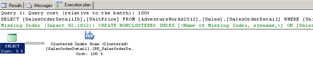
Since the UnitPrice column does not have an index, the clustered index on the primary key (SalesOrderDetailID) had to be scanned. Since there is no ORDER BY clause in our query, the clustered index scan was essentially the same as a table scan. A clustered index is built on the physical leaf pages of a table, so a table with a clustered index will always show a clustered index scan rather than a table scan in an execution plan – even if the two have the same query cost.

To help us with our testing as we compare the impact of creating new indexes, I’ve created a copy of the AdventureWorks2012 database, called AdventureWorks2012b.

Before we create a filtered index, let’s create a traditional nonclustered index on the UnitPrice column of the AdventureWorks2012b database’s Sales.SalesOrderDetail table, and see how that improves our query. We’ll compare the performance of a nonclustered index against the performance of a filtered nonclustered index – the query engine suggests that a nonclustered index could improve the query by over 92%.

Now let’s compare the query execution for both tables, in one batch:

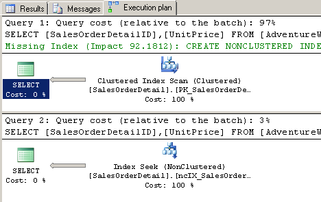
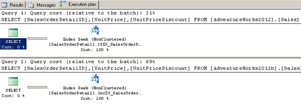
It’s obvious that the introduction of a simple nonclustered index did improve our query by more than 90%. Since nonclustered indexes refer to the primary key (if it exists) of a table, our query did not incur a key lookup. A key lookup is an expensive operation what occurs when a column is included in the SELECT list of a query, but is not covered by an index.

Now let’s add a filtered index to the original table (AdventureWorks2012). The filtered index will be identical to the nonclustered index, with the addition of a WHERE clause. Let’s allow the WHERE criteria to search for UnitPrice values that are greater than $1000:

Now we’ll run our batch query execution again:

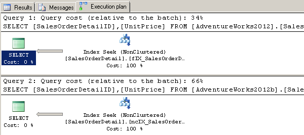
We have reduced our query cost by almost ½ – using a filtered index instead of a traditional nonclustered index.

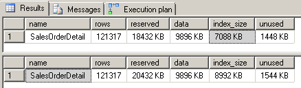
Let’s take a look at the storage cost difference of using a filtered index. By running the sp_spaceused stored procedure, we can find the difference:

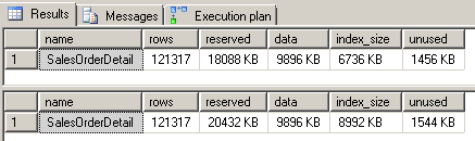
The ‘index_size‘ data was the same for both databases before we added any indexes. We see that by using a filtered index, we’ve saved a considerable storage percentage – about 25%. Of course, the storage savings results of implementing a filtered index will vary depending on the selectivity of the index’s data.

Selectivity

Selectivity could be defined as “the percentage of matching rows compared to total rows, regarding a given query’s criteria.” A lower percentage indicates higher selectivity. This means that if there are very few rows that meet a query’s (or an index’s, in the case of a filtered index) WHERE criteria compared to the total number of rows, the index is considered very selective. For example, unique data would provide the most selective results, while a table that has the same value for every row would be considered least selective. So, if we were to broaden the search criteria of our filtered index like this:

…the index size of the filtered index would be increased:

Sparse columns

Sparse columns are perfect candidates for filtered indexes. Sparse columns offer very efficient storage for columns that contain many NULL values – using no storage space whatsoever for the actual NULL data values. A sparse column must be nullable, and should be used for data where it is expected that the data will be mostly NULL values. A table that contains a sparse column can be created like this:

A filtered index that would work well for the sparse Email column in this table might look like this:

The index will ensure that query time is not wasted on the records with NULL email addresses.

Unique filtered indexes

Filtered indexes are a good solution in a situation where all column data must be unique – with the exception of NULL values. For example, if we want to make sure that all customers use a unique email address if they have one, but still allow the Email column to be NULL, we can use a UNIQUE filtered index:

A traditional nonclustered UNIQUE index will allow only one NULL value. By using a filtered UNIQUE index, we allow multiple NULL Email records, while still guaranteeing that all other Email values will be unique.

Include clause

Filtered indexes offer the added benefit of an optional INCLUDE clause. Using an INCLUDE clause in a nonclustered index provides the ability to cover additional columns in a query’s SELECT list without needing to access a clustered index to access those columns. Therefore, the index can be utilized by wider queries without incurring additional key lookup costs. Let’s demonstrate the use of the INCLUDE clause. If we decide that we also want to return the UnitPriceDiscount field in our SalesOrderDetail query batch, neither of our indexes would be utilized:

The addition of the UnitPriceDiscount column in the select list has caused our nonclustered indexes to be ignored. However, if we add an INCLUDE clause to each index, we can return to similar query cost results:

We’ve expanded the capabilities of our index to cover the UnitPriceDiscount column. Our query that contains UnitPriceDiscount in the SELECT list is now optimized.

Advantages of using filtered indexes

Some key benefits of using filtered indexes are:

• Reduced index maintenance costs. Insert, update, delete, and merge operations are not as expensive, since a filtered index is smaller and does not require as much time for reorganization or rebuilding.
• Reduced storage cost. The smaller size of a filtered index results in a lower overall index storage requirement.
• More accurate statistics. Filtered index statistics cover only the rows the meet the WHERE criteria, so in general, they are more accurate than full-table statistics.
• Optimized query performance. Because filtered indexes are smaller and have more accurate statistics, queries and execution plans are more efficient.

Limitations

Some limitations on using filtered indexes are:

• Statistics may not get updated often enough, depending on how often filtered column data is changed. Because of how SQL Server decides when to update statistics (when about 20% of a column’s data has been modified), statistics could become quite out of date. The solution to this issue is to set up a job to run UPDATE STATISTICS more frequently.
• Filtered indexes cannot be created on views. However, a filtered index on the base table of a view will still optimize a view’s query.
• XML indexes and full-text indexes cannot be filtered. Only nonclustered indexes are able to take advantage of the WHERE clause.
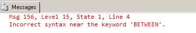
• The WHERE clause of a filtered index will accept simple predicates only. For example,
  1 2 3 4 5

  --add nonclustered filtered index to ModifiedDate column CREATE NONCLUSTERED INDEX fIX_SalesOrderDetail_ModifiedDate ON AdventureWorks2012.Sales.SalesOrderDetail(ModifiedDate) WHERE ModifiedDate BETWEEN '2008-01-01' AND '2008-01-07' GO

  …results in an error:

  

  ..but this:

  1 2 3 4 5

  --add nonclustered filtered index to ModifiedDate column CREATE NONCLUSTERED INDEX fIX_SalesOrderDetail_ModifiedDate ON AdventureWorks2012.Sales.SalesOrderDetail(ModifiedDate) WHERE ModifiedDate >= '2008-01-01'  <= '2008-01-07' GO

  …is accepted. Using date functions also results in an error:

  1 2 3 4 5

  --add nonclustered filtered index to ModifiedDate column CREATE NONCLUSTERED INDEX fIX_SalesOrderDetail_ModifiedDate ON AdventureWorks2012.Sales.SalesOrderDetail(ModifiedDate) WHERE ModifiedDate  = GETDATE() GO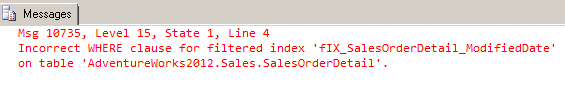

  

  Computed, spatial, and UDT columns are also not allowed as comparison criteria. The IN clause is allowed.

How to know when a filtered index is needed

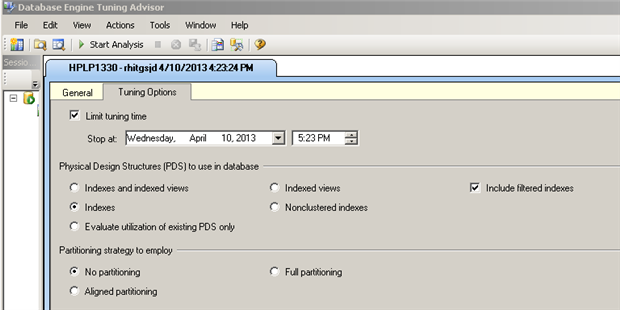
There are obvious benefits to using filtered indexes, but how can we know if certain queries are used often enough to warrant a filtered index? One way to know this is to be intimately aware of the exact queries that are used – by using SQL Profiler to capture query text, or by examining often-used stored procedures and application code. Another method is to use the Database Tuning Advisor. The Database Tuning Advisor offers missing index suggestions, based on a workload file or table. The workload is normally the results of a SQL Server Profiler trace that is consumed and examined. The Tuning Advisor evaluates what queries are executed and how often, and decides if a database table might benefit from additional indexes. The Advisor can be started from Management Studio by selecting Database Tuning Advisor from the Tools menu. Then, in the Tuning Options tab, there is a checkbox labeled ‘Include filtered indexes’ – when this is checked, the Advisor will recommend filtered indexes, where beneficial.

Conclusion

Filtered indexes offer great benefits in terms of query execution performance and index storage savings. Because traditional nonclustered indexes are so necessary, but can rack up high maintenance and storage costs, the filtered index optimization should be considered wherever possible. However, care should be taken not to eliminate any current nonclustered indexes that cannot easily be replaced with filtered indexes.