Introduction

There are a lot of Multidimensional Expressions (MDX) resources available, but most teaching aids out there are geared towards professionals with cube development experience. As a result SQL developers with no cube development experience start learning MDX on a poor footing because many of the learning aids completely disregard SQL as a good frame of reference for starting the learning process.

I am going to introduce MDX by drawing only on the similarity and differences between MDX and SQL and more importantly tackle some core MDX and cube concepts along the way.

In this first part, I will explain how to navigate the cube object with MDX by cutting through some of the quirkiness that makes MDX different from T-SQL even though both were are derived from SQL language.

Before we move on let’s see how SQL Server 2012 is changing SQL Server data analytics and why MDX is still very important in that regard. 

Role of MDX in SQL Server Analytics today

With the introduction of SQL Server 2012 and the Analysis Services BISM now introduces two models yhr Multidimensional and the Tabular Model. You can read about them here: http://www.microsoft.com/sqlserver/en/us/solutions-technologies/business-intelligence/SQL-Server-2012-analysis-services.aspx.

MDX is the primary language used to query cubes built on the Multidimensional models and is still unsurpassed in many areas when it comes to data analysis. It is also currently the only language that can query both the Tabular and Multidimensional models in SQL Server 2012. It is also the language for most front end applications including third-party ones and the popular Excel which can connect to PowerPivot and the two models in SQL Server 2012. I am not evangelizing for MDX or starting a debate, I am just pointing out a few of its benefits in light of this topic.

Prerequisites

I am going to use the SQL Server 2008 Adventure Works cube and the SQL Server 2008 AdventureWorksDW relational database for all MDX and SQL queries respectively. To be able to follow the example you must be able to connect to the the cube and data warehouse and run the queries under each section. For the download and installation of the AdventureWorksDW relational database and Adventure Works cube you can check out this site http://www.ssas-info.com/analysis-services-faq/29-mgmt/242-how-install-adventure-works-dw-database-analysis-services-2005-sample-database

How is a relational database different from a cube?

If you are reading this you probably know that SQL is used to query relational databases and tables are the basic objects that we query in relational databases. From the previous section we learned that MDX is primarily used to query cubes build on Multidimensional models. Another thing you need to know is that, like tables in relational databases the basic objects that you will query in the cube are called dimensions.

If you have no cube development experience don’t worry because from the perspective of the SQL and the MDX languages there is not much difference between a cube and relational database. Table1 below shows the parallels between a relational database and cube from the perspective of the two languages.

Table 1: showing the basic parallels between a relational database and a cube from the perspective of SQL and MDX Languages.

In a summary:

1. The equivalent of a database table in a cube is called a dimension.
2. T-SQL (SQL) queries database tables, MDX queries dimensions.

Note also that tables are transformed directly into in dimensions during the cube building process.

To further illustrate these points let’s look at figure 1 below. The figure shows a simple but exact mapping of how some five tables in the AdventureWorksDW  relational database are represented as dimensions in the Adventure Works cube, with the exact names used in both environments. You can also see how the columns in the tables are represented as attributes in the cube.

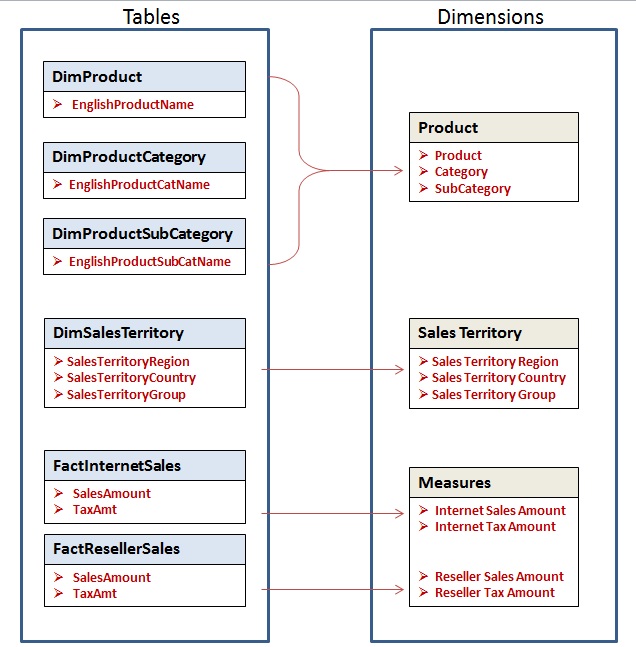
Fig1:  Shows how  tables in the "AdventureWorksDW" relational database translate into dimension in the "Adventure Works" cube use for demos in this document.

There are a few things you should note in the mapping figure1 above.

• The cube maintains one “special” dimension it calls Measures. This special dimension holds numerical data (counts, amounts etc.) normally referred to as measures. In the relational database, the tables that hold the measures that feed the Measures dimension are called Fact tables. They are normally identified as “fact” tables either by schema or by naming conventions. For e.g. in figure1, all the tables mapped into the Measures Dimension come from relational tables with names prefixed with “Fact” (dbo.FactResellerSales, dbo.FactInternetSales)
• All the “not so special” dimensions in the cube are referred to as “Regular” dimensions and are populated with textural data relating to the measures. In the relational database, the tables that hold the data that feed the Regular dimensions are called dimension tables and are normally identified with “Dim” either by schema or by naming conventions. For e.g. in figure1, all the tables mapped into the Regular dimensions in the cube have names prefixed with “Dim” (dbo.DimSalesTerritory dbo.DimProduct, dbo.DimProductCategory and dbo.DimProductSubCategory).
• Data mapped into a dimension can come from one or more tables as you can see from the product Dimension.

Going forward I will refer to the AdventureWorkDW relational database as the “database” and the Adventure Works cube as the “cube”.

Basic SQL Syntax

MDX like T-SQL revolves around the general SQL syntax. I am going to look at the differences and similarities between the two languages by looking at clauses in the general SQL syntax below. I am not going to introduce the clauses in query execution context or in any particular order.

SELECT <select_list>

FROM <left table> join<right_table>

WHERE <where_predicate>

GROUP BY <group_by_specification>

HAVING <having_predicate>

ORDER BY <order_by_list>;

Using the tables-to-dimensions mapping illustrations in figure1, let's explore the similarities and differences between MDX and SQL by looking at each Clause. Remember, I will mostly use the tables and dimensions in the illustrations in the figure1 for most of our initial SQL and MDX queries.

The "SELECT" and "FROM" Clauses

From figure1, let’s say we want to retrieve the Internet Sales Amount. In the database that will be the column SalesAmount in the FactInternetSales table, and in the cube that will be InternetSaleAmount attribute in the Measures dimension.

In SQL we select SalesAmount directly from the FactInternetSales table to retrieve the value. On the other hand, in the cube we navigate to the Measures dimension to retrieve values of this attribute.

The SQL and MDX syntaxes to select the same attribute from the two environments are as shown in listing1 below:

Listing1.

SQL:

SELECT [FactInternetSales].[SalesAmount]

FROM [FactInternetSales]

MDX:

SELECT [Measures].[InternetSalesAmount]

FROM [Adventure Works]

The first major difference to note is that in MDX even though the SELECT list are derived from dimensions, the FROM clause is not on the dimension but on the cube, unlike in SQL where the FROM clause is directly on tables. Generalized syntaxes showing this major difference is as below.

SQL:

SELECT [Table].[ColumnName]

FROM [Table]

MDX:

SELECT [Dimension].[AttributeName]

FROM [Cube]

Display Axis

If you run MDX query in listing1 above it will fail but if you modify it by adding the clause “ON COLUMNS” to the select list as shown in listing2 below then it will succeeds.

Listing2.

MDX:

SELECT [Measures].[Internet Sales Amount] ON COLUMNS                                      FROM [Adventure Works]

This clause is required because MDX can display result on more than the regular COLUMNS and ROWS axes that we are used to in SQL. As a result, MDX requires that you always specify a display axis for all elements in the SELECT list.

Listing3 and Listing4 below show further examples of how elements in the MDX SELECT list may be displayed on different Axes.

Listing3. Showing two attributes displayed on one axis

MDX:

SELECT (

[Measures].[Internet Sales Amount]

,[Product].[Product]

) ON COLUMNS

FROM [Adventure Works]

Results:

Listing4. Showing two attributes each displayed on a different axis

MDX:

SELECT

   [Measures].[Internet Sales Amount] ON COLUMN

   ,[Product].[Product] ON ROWS

FROM [Adventure Works]

Results:

The query in Listing4 show explicit display on two axes namely COLUMNS and ROWS.   The COLUMNS and ROWS names are actually aliases for the true names of two of many MDX axes namely, Axis (0), and Axis (1) respectively. So instead of using the COLUMNS and ROWS aliases as in Listing4 above you can also the actual axis numbers as below;

MDX1:

SELECT [Measures].[Internet Sales Amount] ON axis(0)

, [Product].[Product] ON Axis(1)

FROM [Adventure Works]

Or

MDX2:

SELECT [Measures].[Internet Sales Amount] ON 0

, [Product].[Product] ON 1

FROM [Adventure Works]

MDX query can have up to 128 axes, with alias names for a few of them. Most professional MDX queries are restrict display to two axes, so we are also going to stick to only the first two axes. We will also stick to using the COLUMNS and ROWS axis aliases for the axis 0 and 1 respectively as shown in Listing3 and Listing4

Remember that you cannot skip axis, in other words you cannot display on axis(1) displaying on axis(0) first. If you don’t to display anything on axis you can display an empty set { } as below.  

MDX2:

SELECT

 {} ON ROWS

, [Product].[Product]  ON COLUMNS

FROM [Adventure Works]

If you are not following these examples, be careful when select more than one attribute on an axis, MDX uses brackets and concept of dimensionality to control how multiple items are displayed on an axis. Due to the importance I will dedicate a chapter to talk about it later.

JOINS

Now let’s see how MDX handles Joins. Let’s say in addition to the Internet Sales Amount we retrieved in listing1, we want to retrieve Sales Territory Region as well. In the Database, we now navigate to both columns by joining two tables namely DimSalesTerritory and FactInternetSales by using “JOIN” word in the query.

In the cube we also navigate to two different dimensions namely Measures and Sales Territory because the Internet Sales Amount and the Sales Territory Region attributes are mapped separately those two dimensions. However, in MDX we don’t need to use the “JOIN” word, the cube already has information as to how the two dimensions are to be joined as part of its metadata definitions. The SQL and MDX syntaxes and query results are as showed in Listing5 below.

Listing5

SQL:

SELECT

    [DimSalesTerritory].[SalesTerritoryRegion]

    ,[FactInternetSales].[SalesAmount]
FROM FactInternetSales

INNER JOIN DimSalesTerritory
ON FactInternetSales.SalesTerritoryKey = DimSalesTerritory.SalesTerritoryKey

Result:

.................

MDX:

SELECT

  [Measures].[Internet Sales Amount] ON COLUMNS

  ,[Sales Territory].[Sales Territory Region] ON ROWS

FROM [Adventure Works]

Result:

Another major difference between SQL and MDX is the fact that unlike SQL, MDX does not need to explicitly join dimensions using the "JOIN" word when pulling data from multiple dimensions. You always select FROM the cube and the cube does all the Joining for you. A generalized SQL and MDX syntax are shown below.

Listing6. General Syntax

SQL:

SELECT

   [Table1].[ColumnName]

  ,[Table2].[ColumnName]

FROM [Table1] join [Table2]

MDX:

SELECT

    [Dimension1].[AttributeName] ON axis   

   ,[Dimension2].[AttributeName] ON axis

FROM [Cube]

Aggregation and "GROUP BY" Clause

Looking at the result from the two queries in listing5 in the previous section, you probably realized that the output in the result set from the MDX and SQL queries are not the same even though they are retrieving the same mapped items. So why is it that the same mapped items are returning different set of records? To answer this question let’s do two things,

1. Take the SQL query from the previous section and apply the SUM aggregation function and Group By clause to it.
2. Modify the MDX query from the previous section by repeating the SalesTerritoryRegion attribute name like this:[SalesTerritoryRegion].[SalesTerritoryRegion]

The modified versions of the logic are shown in Listing6 below.

Now when you run the two modified query, except for a null value in the MDX result, the two result set should match as shown in the results from the modified queries in Listing5 below.

Listing6;

SQL:

SELECT

  Sum([FactInternetSales].[SalesAmount]) as SalesAmount

  ,[DimSalesTerritory].[SalesTerritoryRegion]
FROM FactInternetSales

INNER JOIN DimSalesTerritory

ON FactInternetSales.SalesTerritoryKey = DimSalesTerritory.SalesTerritoryKey
GROUP BY [DimSalesTerritory].[SalesTerritoryRegion]

Result:

MDX:

SELECT

   [Measures].[Internet Sales Amount] ON COLUMNS

  ,[Sales Territory].[Sales Territory Region].[Sales Territory Region] ON ROWS
FROM [Adventure Works]

Result:

There are a few things happening here. First, MDX by default always implicitly aggregates the attributes in the Measures dimension (in this case Internet Sales Amount) and implicitly group the result by any other Dimensional Attribute in the SELECT list. The aggregation function it applies (in this case "SUM") is defined at design time. In other words, every Attribute in the Measures dimension is assigned an aggregate function at design time which is by default applied in the MDX queries.

On the other hand SQL will return detail records unless you explicitly tell it to aggregate the data by including a specific aggregate function and the Group By clause.

Attribute Hierarchies

You might be wondering why we repeated the name of the SalesTerritoryRegion Attribute like this [Sales Territory Region].[Sales Territory Region] in Listing5

Let’s look at the Sales Territory dimension again, fig3 below show Sales Territory dimension as presented in the initial mapping in figure1.

Fig 3. Showing Sales Territory Table-Dimension Mapping

What is not shown is the fact that by default the cube actually creates a hierarchy out of each attribute that is mapped into a Regular dimension. Figure4 below shows a drill down of each of the attribute in the Sales Territory dimension displaying the two-level hierarchy under each attribute.

Figure4: Shows a drill-down look into the Sales Territory dimension Attribute Hierarchy.

Each attribute hierarchy as we will now refer to them consists of a top level member called "All" and an Attribute level (with the same name as the name of the attribute hierarchy) below it. Note that some of these default behaviors may be modified in many ways at design time. For Instance the “All” member name can be changed, in AdventureWorks it was changed to “All Sales Territories” which is more appropriate.

This means that to navigate to each attribute level in other to display all detail level data, you have to navigate to the dimension, the Attribute Hierarchy and then the attribute level, all by name as shown below.

[<Dimension Name>].[<Hierarchy Name>].[<Level Name>]

Listing7 below for instance shows how to navigate to the Sales Territory Group and Sales Territory Region attribute level in the SELECT list to obtain the detailed records of these attribute in both SQL and MDX.

Listing7:

MDX:

SELECT {} ON COLUMNS

,(

      [Sales Territory].[Sales Territory Group].[Sales Territory Group]

      ,[Sales Territory].[Sales Territory Region].[Sales Territory Region]

) ON ROWS

FROM [Adventure Works]

Result:

SQL:

SELECT

   [DimSalesTerritory].[SalesTerritoryGroup]

  ,[DimSalesTerritory].[SalesTerritoryRegion]

FROM DimSalesTerritory

Result:

Introduction to MDX Functions

As we saw from the previous section the cube turns dimensional attributes into hierarchies. Let’s see how a cube implements a dimension. Figures4 below shows a detail level representation of the Sales Territory dimension and the three independent attribute hierarchies creates under it.

Fig3. Showing detail implementation of the 3 Attribute Hierarchies and levels in the Sales Territory Dimension      

Beside these default attribute hierarchies created by the cube, the cube permits developer to create their own hierarchies called user-defined hierarchies with as many levels as they want.

Creating hierarchical structures allows the cube to navigate to the different levels of the dimensions quickly, and by the use of functions like members, children, siblings, cousin, ancestors, descendants it know where to go and what to retrieve.

Note that the bulk of the complexity of MDX is to do with navigating and retrieving data subset at different levels in hierarchies and finally combining and manipulating these subsets of data, so it is worth understanding cube hierarchies. Let’s look at some simple hierarchy functions.

The  Members Function

Members are items under a dimension, hierarchy or level. The members function returns a set that represents all of the members in the level (dimension, hierarchy, or level) that it is applied. Below are examples of the use of the member function

Example 1: members function applied at the Attribute hierarchy level.

MDX:

SELECT

    {} ON COLUMNS

  ,[Sales Territory].[Sales Territory Group].members

ON ROWS

FROM [Adventure Works]

Result:

Note that the “All Sales Territory” in the cube member is returned in the result set.

Example 3: members function applied at the Attribute level.

MDX:

SELECT

   {} ON COLUMNS

  ,[Sales Territory].[Sales Territory Group].[Sales Territory Group].members

ON ROWS

FROM [Adventure Works]

Result:

Note that the “All Sales Territory” member was not returned in the result set.

The Children function

The children function returns a set that contains the children of a specified member. If the specified member has no children, this function returns an empty set.

Note that in attribute hierarchies it is only the hierarchy level member that has children.

MDX:

SELECT

{} ON COLUMNS

,[Sales Territory].[Sales Territory Group].children ON ROWS

FROM [Adventure Works]

Results:

Note that the “All Sales Territory” member is not returned because it not an actual child. It is a member created to represent the Total of all the children as shown when we add a measure to the query with the member function as shown below. The amount “$80,450,596.98” is the total of all the children.

MDX:

SELECT

    [Measures].[Reseller Sales Amount] ON COLUMNS

  ,[Sales Territory].[Sales Territory Group].members

ON ROWS

FROM [Adventure Works]

Results:

You can retrieve only the “All Sales Territory” member by referencing it as below.

MDX:

SELECT

    [Measures].[Reseller Sales Amount] ON COLUMNS

  ,[Sales Territory].[Sales Territory Country].[All Sales Territories]

ON ROWS

FROM [Adventure Works]

Result:

In this section we looked at attribute hierarchies and some simple functions. We will explore User-defined hierarchies and some more functions later on in this series.

The “WHERE” Clause

Now, let’s say we want to restrict Internet Sales Amount to where Sales Territory Group is Europe. As shown in listing9 below, MDX uses Dot Notations in the where clause as oppose to the equal to sign used in SQL.

Listing9:

SQL:

SELECT sum(dbo.FactInternetSales.SalesAmount) as InternetSalesAmount

FROM dbo.FactInternetSales

INNER JOIN dbo.DimSalesTerritory

ON dbo.FactInternetSales.SalesTerritoryKey = dbo.DimSalesTerritory.SalesTerritoryKey

WHERE dbo.DimSalesTerritory.SalesTerritoryGroup='Europe'

Result:

MDX:

SELECT

   [Measures].[Internet Sales Amount] ON COLUMNS

FROM [Adventure Works]

WHERE [Sales Territory].[Sales Territory Group].[Europe]

Result:

Now let’s say we want to display the Sales Territory Group as part of the result set. If you are from SQL background the natural incline will be to add the Sales Territory Group to the select list as shown in listing10. for both SQL and MDX.

listing10:

SQL:

SELECT

dbo.DimSalesTerritory.SalesTerritoryGroup

,sum(dbo.FactInternetSales.SalesAmount) as InternetSalesAmount

FROM dbo.FactInternetSales

INNER JOIN dbo.DimSalesTerritory

ON dbo.FactInternetSales.SalesTerritoryKey = dbo.DimSalesTerritory.SalesTerritoryKey

WHERE dbo.DimSalesTerritory.SalesTerritoryGroup='Europe'

GROUP BY dbo.DimSalesTerritory.SalesTerritoryGroup

Result:

MDX:

SELECT

 [Measures].[Internet Sales Amount] ON COLUMNS

 ,[Sales Territory].[Sales Territory Group].[Europe] ON ROWS

FROM [Adventure Works]

WHERE [Sales Territory].[Sales Territory Group].[Europe]

   result:

Error: The Sales Territory Group hierarchy already appears in the Axis0 axis.

But when you execute the MDX version it will fail as shown in the MDX result in listing 10 above.

The Problem is that, In MDX the dimension on the WHERE clause acts as what is called a “slicer dimension”. In other words they are dimensions that are not explicitly assigned to an axis and so MDX sees it as repeating SalesTerritoryGroup dimension attribute.

Instead, let’s move the dimension into the select list without the WHERE clause as shown in listing11 below. Now when you run the modified query, the right result, similar to the SQL version is produced. As shown in the result in listing11 below.

Listing11:

MDX :

SELECT

[Measures].[Internet Sales Amount] ON COLUMNS

,[Sales Territory].[Sales Territory Group].[Europe] ON ROWS

FROM [Adventure Works]

Result:

Note that there some implications in choosing where to add dimension members i.e. whether to the WHERE clause or directly on the Axis. This is because in the context of MDX query execution, MDX resolves the WHERE phase before processing dimensions on the display Axis.

Emerging from this section what did we learn? We learned that “WHERE” Clauses acts as filters in SQL but as a Slicer dimension in MDX.

There is an actual “Filter" clause in MDX we will later see some Filter function example after we’ve looked at some other MDX concepts.

The “HAVING” Clause

For Sample queries of how the HAVING expressions is used in both SQL and MDX, lets once again retrieve the Sales Territory Groups where Internet Sales Amount is greater than $9M. The SQL and corresponding MDX queries and theirs results are shown below are shown in listing12 below. 

Listing12:

SQL:

SELECT

 [DimSalesTerritory].[SalesTerritoryGroup]

 ,Sum([FactInternetSales].[SalesAmount]) as SalesAmount

FROM FactInternetSales

INNER JOIN DimSalesTerritory

ON FactInternetSales.SalesTerritoryKey = DimSalesTerritory.SalesTerritoryKey

GROUP BY [DimSalesTerritory].[SalesTerritoryGroup]

HAVING Sum([FactInternetSales].[SalesAmount])>9000000

Result:

MDX:

SELECT

      [Measures].[Internet Sales Amount] ON COLUMNS  

      ,[Sales Territory].[Sales Territory Group].[Sales Territory Group]

HAVING [Measures].[Internet Sales Amount]>9000000 ON ROWS

FROM [Adventure Works]

Result:

This example returns only the Sales Territory Groups where Internet Sales Amount is greater than $9M.

Let’s look at the MDX query. Note that unlike the "WHERE" clause, the "HAVING" clause is treated as an actual filter in MDX. But unlike the WHERE clause it is used to filter the contents of an axis based on defined criteria.

Note that have some implications in its application since dimensions on different axes are evaluated independently, before their intercepting cells are evaluated.

Even though options like the FILTER function might be more flexible to use, "HAVING" expressions could be simpler if you are conversant with them.

Ordering

MDX arranges members of a specified set so it uses an “ORDER” clause as oppose to “ORDER BY” in SQL. Ordering in SQL is straight forward as seen in the before and after SQL queries below.

SQL1:

SELECT

  [DimSalesTerritory].[SalesTerritoryRegion]

  ,Sum([FactInternetSales].[SalesAmount]) as SalesAmount

FROM FactInternetSales

INNER JOIN DimSalesTerritory

ON FactInternetSales.SalesTerritoryKey = DimSalesTerritory.SalesTerritoryKey

GROUP BY [DimSalesTerritory].[SalesTerritoryRegion] 

SQL2:

SELECT

  [DimSalesTerritory].[SalesTerritoryRegion]

  ,Sum([FactInternetSales].[SalesAmount]) as SalesAmount

FROM FactInternetSales

INNER JOIN DimSalesTerritory

ON FactInternetSales.SalesTerritoryKey = DimSalesTerritory.SalesTerritoryKey

GROUP BY [DimSalesTerritory].[SalesTerritoryRegion]                          ORDER BY  Sum([FactInternetSales].[SalesAmount]) desc

Result:

Now let’s look at how the MDX ORDER function works by looking at an ordered and unordered MDX versions of the SQL query above.

MDX1: UnOrdered

SELECT

[Measures].[Internet Sales Amount] ON COLUMNS

,[Sales Territory].[Sales Territory Region].[Sales Territory Region]

ON ROWS

FROM [Adventure Works]

Result:

MDX2: Ordered

SELECT

[Measures].[Internet Sales Amount] ON COLUMNS

,ORDER

(  [Sales Territory].[Sales Territory Region].[Sales Territory Region]

  ,[Measures].[Internet Sales Amount]

  ,DESC

)

ON ROWS

FROM [Adventure Works]

Result:

From the ordered MDX query we can see that the ORDER function takes three arguments as below.

ORDER (Set, Expression, Flag)

Notice that Sales Territory Region is being ordered by Internet Sales Amount. Because of that Internet Sales Amount is included as the second argument in the ORDER function even though it is not being displayed on the ROWS axis. The third argument is the flag indicating the sorting order.

Initial Sets

Run MDX1 and MDX2 queries below.

Looking at the queries and the result sets you will notice that even though Reseller Sales Amount measure is not specified in the SELECT list in MDX2 the results returns that measure, similar to MDX1 where the Reseller Sales Amount measure is explicitly requested in the SELECT list.

MDX1:

SELECT

[Sales Territory].[Sales Territory Country].[All Sales Territories] ON COLUMNS

,[Measures].[Reseller Sales Amount] ON ROWS

FROM [Adventure Works]

Result:

MDX2:

SELECT

[Sales Territory].[Sales Territory Country].[All Sales Territories] ON COLUMNS

FROM [Adventure Works]

Result:

Now run MDX3 below and notice that this time nothing was provided on the SELECT list but the cube still returns that same figure $80,450,596.98 as in the previous two queries.

MDX3:

SELECT

FROM [Adventure Works]

Result:

We know that if you try running any SQL query with no items on the SELECT list the query will fail so why is the MDX3 returning any results at all?

The difference is that SQL start with an empty set and then populates this empty set based on request on the select list. On the other hand MDX starts with a default populated set and slice and dice this initial set with your request on the slicer dimensions on your WHERE clause and the SELECT list on your axes.

In MDX the initial set consist of default attribute members of all the dimensions defined at design time. For instance in the cube, Reseller Sales Amount was defined as the default attribute members of the Measures dimension by the creator of the cube.

By default the cube will return this Reseller Sales Amount measure if you don’t specify any measure in your query as we saw in MDX2 and MDX3 above.

The only way to avoid the default measure being returned is by specifying  a different measure, for instance selecting Internet Sales Amount  as shown in MDX4 or explicitly returning an empty sets as shown in MDX5 below.

MDX4:

SELECT [Measures].[internet Sales Amount] ON COLUMNS

FROM [Adventure Works]

Result:

MDX5:

SELECT {} ON COLUMNS

FROM [Adventure Works]

.DefaultMember Function

You can check the default attribute member of any dimensional attribute by using the .DefaultMember function. The general syntax for doing that is:

Dimension.hierarchy.DefaultMember

or

Dimension.DefaultMember (for the Measures Dimension which does not have hierarchies)

By running MDX1 below we can verify that the Reseller Sales Amount is indeed the default attribute of the Measures dimension.

 MDX1:

select

  Measures.DefaultMember ON COLUMNS

FROM [Adventure Works]

Result:

We can also verify that the All Sales Territories member is the default member of the Sales Territory Country by running MDX2 below.

MDX2:

SELECT

  Measures.DefaultMember ON COLUMNS

  , [Sales Territory].[Sales Territory Country].DefaultMember ON ROWS

FROM [Adventure Works]

Result:

MDX and the Tabular model

In the beginning I mentioned that MDX can query cubes developed on both the Tabular and Multidimensional models. Queries MDX1 and MDX2 below returns the same result set when run against SQL Server 2012 Tabular and Multidimensional model cubes respectively. Note that the only differences between the two queries are the cube names and the measure names, because they were named differently in the two models.

MDX1:

//AdventureWorks 2012 Tabular

SELECT

       [Measures].[Internet Total Sales] ON COLUMNS

       ,[Sales Territory].[Sales Territory Group].members ON ROWS

FROM [Internet Sales]

MDX2:

//AdventureWorks 2012 Multidimensional

SELECT

       [Measures].[Internet Sales Amount] ON COLUMNS

       ,[Sales Territory].[Sales Territory Group].members ON ROWS

FROM [Adventure Works]

Result:

Summary

We have seen how to navigate the cube to retrieve certain Data elements by comparing MDX compares to SQL. We’ve also seen that MDX could be less  “complicated” in some regards, for instance in MDX you don’t have to worry about "Joins". Like I said earlier most of the complexities of MDX is do with hierarchies and resolving sets on different axes.

In this Part, I restricted MDX query to simple examples till we discuss some very important cube concepts like dimensionality, slicing and user-defined hierarchies. However every query we will later write revolves around what has been introduced here. Also Just as SQL Functions augments the basic syntax, so does all MDX functions we will learn later learn augment what has been introduced here.

Next Steps

We will look at how to use brackets, and the concept of dimensionality to control and properly format the SELECT list on each display axis. We will also explore user-defined hierarchies some more MDX functions.