by Steve Bolton
The data mining method known as Time Series is aptly named, because it seems to take a long series of time to get it right.
Out of the nine algorithms included in SQL Server Data Mining (SSDM), Time Series is on a par with Neural Networks in terms of sophistication, raw power and potential usefulness. When properly designed, neural nets can also be used to predict future trends based on past data, but Time Series is usually the preferred tool when projecting slices of time with definite intervals; its inner workings are also complex but still far easier to interpret than the innards of neural nets, as explained in A Rickety Stairway to SQL Server Data Mining, Algorithm 5: The Neural Network Algorithm. Sequence Clustering is the only other SSDM algorithm that is implicitly temporal, but it can also be applied to data that is ordered but not in terms of time – one of its most common applications is in gene sequencing, for example. That algorithm is usually applied to slices of time that are indefinite, which might make it an ideal choice for a DBA to harvest Windows and SQL Server log data for sporadic server events. Like Sequence Clustering and Association Rules, Time Series has a fairly long learning curve, which is another reason why I saved it for the end of this segment of my self-tutorials on SSDM. On the other hand, it is a much more versatile tool, in that it has far fewer restrictions on input data than many of the other algorithms and can be applied to a much wider range of temporal problems. Certain other algorithms like Clustering, Naïve Bayes and Logistic Regression can only be applied to temporal projections in an awkward way, while with Association Rules you might as well banish the thought of using it to accurately predict the future, because it’s not going to happen. Linear Regression and Decision Trees can be used for predictions, but SQL Server data miners might as well use Time Series if they have the computational resources, given that it uses both of these algorithms as building blocks to make predictions with much greater accuracy.
As always, I preface my articles with a disclaimer that I’m posting this series in order to learn the ropes, while providing some badly needed publicity to the most under-utilized tool in SQL Server; if even an amateur like myself can use it to uncover profitable hidden relationships in data, then real DBAs can probably gain even more from it with minimal expenditures of time, training and server resources. On the other hand, I do have real expertise in history, including a Master’s degree and part of a doctorate. I remember getting into debates with other grad students about the purposes of history, where I took the sometimes unpopular stance that the chief use of the past is to affect the future. The past may have some intrinsic value of its own, but history is mainly antiquarian entertainment unless it is used to fix today’s problems tomorrow. Perhaps that is because I specialized in foreign policy, which is an area where forecasting is crucial, for the simple reason that people die in large numbers when our statesmen fail to learn from history. I tend to look at data from the same philosophical viewpoint. All of those numbers and letters DBAs toil to preserve are already part of the past, and their chief use is to apply them to tomorrow’s challenges. This is true of OLTP as well as OLAP data; one saves yesterday’s records to make them available for tomorrow’s transactions, while the other analyzes the patterns from one year’s records to forecast the challenges an organization will face the next year. Yesterday’s data makes tomorrow’s action possible. Time Series is one of the most valuable data mining algorithms precisely because it is more explicitly in line with this goal than some of its competitors. It is not necessarily a “better” mining method though. With data mining, matching the proper tool with the right task is a critical question, and Time Series is not always the best choice. You wouldn’t use it to divide data into groups based on characteristics that have nothing to do with time, in which case you’re better off using Clustering or Association Rules, or another preliminary algorithm like Naïve Bayes. A common design pattern in data mining, however, is to use non-temporal algorithms like these to identify groups, then use Time Series to see how they change over the course of a series of precise intervals. This is the basically the workflow I’ve used up until this post, in which we will apply some of the knowledge gained from the other algorithms to temporal predictions. When it is used in this way, the types of data that Time Series can operate on are bounded only by human imagination, as long the intervals we’re predicting are specific. For a long list of the many varied applications Time Series is put to today, see the Wikipedia page on the topic. Earthquake prediction and weather forecasting are among the more glamorous and highly useful applications of Time Series that benefit the human race every day.
The output of Time Series can be interpreted with a fair amount of ease, even by laymen. Just picture a line chart, which for the uninitiated, simply has the time intervals depicted horizontally at the bottom and the values you’re measuring listed vertically on the left side, with one or more lines and curves in the middle to show the trends of your data. For a couple of simple examples, see the webpage 6.4.5.1. Example of Multivariate Time Series Analysis in the National Institute of Standards and Technology’s Engineering Statistics Handbook, which I highly recommend for amateurs like myself who want to learn the basics of stats quickly. Visualizing the results is the easy part. The hard part is explaining the inner workings of the algorithm, which is surpassed in complexity only by neural nets. It may be arcane, but keep in mind, that doesn’t mean it works magic. There is an unspoken tendency among those, like myself, who don’t fully understand the hard-core math behind it all to treat data mining with a touch of superstition, especially when it unearths valuable patterns. This tendency is magnified with Time Series since we’re predicting the future. It is not a black art, although the math behind it may be a black box to those of us without doctorates in stats, which aren’t needed to put SSDM to productive use. Time Series does not receive messages from beyond the mortal plane like St. Odilia or Mother Shipton. Nor does it perform the ex nihilo miracle of adding information out of thin air, which is logically impossible. As explained in A Rickety Stairway to SQL Server Data Mining, Part 0.1: Data In, Data Out, data mining can at best preserve and identify information that is already present in the finite data we feed into it. If we feed Time Series garbage in the form of wrong data, bad data or insufficient good data, we’re basically just projecting garbage into the future. It is not easy to understand how Time Series churns through the data it is fed, but this is mainly because so many separate steps are involved, not because they are beyond the ken of laymen. As mentioned before, the algorithm makes heavy use of Linear Regression and Decision Trees, two statistical building blocks we’ve covered before. If you can follow the explanations in those tutorials, you’re half-way home. If you haven’t gone through them yet, have no fear, it’s not as hard as it sound. Regression is a topic covered in many general math courses at high school senior or freshman college level, while Decision Trees is just an adaptation designed with non-linear data in mind, so that instead of a single line through a scatter plot, you get jagged ones that change course in tandem with the data. Microsoft’s version of Time Series depends on a variant of Linear Regression called auto-regression, which is even simpler in the sense that a single variable is used to calculate its own regression line, rather than its influence on a second variable. It also makes use of moving averages, which seems to be a somewhat advanced but relatively common calculation in relational databases, judging from the fact that it is often included at the tail end of the T-SQL cookbooks I’ve read. I’ve avoided posting equations throughout much of the series, partly because I’ve somehow forgotten half of the math I used to know back when I was in fourth grade, and used to solve equations for my father, a college physics teacher. Secondly, we don’t really need it to use Time Series or any other SSDM algorithm, just as we can drive cars without giving dissertations on automotive engineering first. When driving a car, it is nonetheless helpful to understand basic concepts about what’s going on under the hood, such as what functions pistons serve in the engine. Likewise, the important things to understand in this discussion of the inner workings of Time Series are the functions the statistical building blocks are meant to serve. The equations themselves are secondary because the whole point of SSDM is to implement all of that advanced stuff for you. Chances are if you’re a DBA, you’re already familiar with moving averages, and if you’ve been to college, you’ve been exposed to regression analysis in the past. It only takes one baby step up our rickety stairway to understand that Decision Trees produces a jagged regression line rather than the single straight one Linear Regression puts out, for the purpose of modeling data that doesn’t follow a straight path. All that remains is to explain how these three building blocks are combined together in Microsoft’s implementation of Time Series.
The Wikipedia page on the subject lists scores of different methods of calculating Time Series, which is really a group of related algorithms. As with Clustering, keeping track of all of the research going on in the field would be quite difficult even for an expert, because its many constituent methods are put to diverse and highly specific purposes in widely separated fields that are exceedingly compartmentalized. One of the avenues of research, however, was pioneered by Microsoft itself, through an adaptation of the mining method we discussed in A Rickety Stairway to SQL Server Data Mining, Algorithm 3: Decision Trees. Much of the explanation that follows on the Auto Regression Trees with Cross Predict[ii] (ARTXP) algorithm within Time Series comes from a paper presented in 2002 by three Microsoft statisticians.[iii] It is adept at short-term predictions but not at long-term forecasting, so in SQL Server 2008 Microsoft added an implementation of the industry standard Box-Jenkins method, also known as an Arithmetic Moving Average (ARIMA). Users can set the FORECAST_METHOD parameter to use one or the other exclusively, but in this post I left it at its default value of MIXED. For lack of time I also did not experiment with PREDICTION_SMOOTHING, which can be used to specify how the two algorithms are blended together to produce a single set of outputs in SSDM. The closer the parameter is to zero, the more the results are exponentially weighted in favor of ARTXP, but the closer it is to 1, the more they are weighted towards ARIMA. I am not yet sure if the normalization curve Microsoft uses is applied before or after ARTXP and ARIMA are finished processing Time Series data in their own unique ways. This may be a subject for future experimentation, since a substantial impact on performance may occur if it is applied afterward and weighting turns out to be more costly for one algorithm than the other. Keep in mind that the two algorithms are also always weighted by temporal distance, so that ARTXP figures more prominently in short-term predictions and ARIMA towards long-term ones, assuming that they’re both enabled. Cross-prediction, i.e. forecasting the values of multiple columns so that they take each other’s predictions into account, is only available with ARTXP.[iv] It is also one of many Time Series features that are only available with Enterprise Edition, so it is important to plan for the correct version of SQL Server if your projects require this algorithm.
The aforementioned research paper on ARTXP also mentions Markov models, which are the backbone of Sequence Clustering, but it is unclear to a novice like me from reading the paper if they are actually employed in SSDM. It also mentions that Monte Carlo methods, another common building block in statistics, can be used to interpolate values between leaf nodes in Decision Trees when future values are not known, but again, I’m not sure if it is used in the SSDM implementation or not.[v] As usual, much of the original research paper is over my head, but it isn’t difficult to understand the point of it all. Auto-regression lines are obviously weak tools by themselves, given that the past behavior of a single variable is not necessarily a reliable predictor of how it will behave in the future. Worse still, simple auto-regressions can’t even model non-linear relationships in that single variable.. Without the Decision Trees component of SSDM to conserve and identify it, a lot of the information present in the data would be lost if depicted in a single straight line. The places where the modified auto-regression lines SSDM produces branch off at crooked angles depict places where a pronounced change has taken place in the data. If the change occurs in the temporal values used as the key it “means that there is a change in the trend at a certain point in time.”[vi] If there are no splits in the results SSDM returns, then what we’re left with is basically a simple auto-regression.[vii]
It’s not quite this simple as this, but much of the added complexity in ARTXP and ARIMA comes from merely tacking additional terms on the end of regression formulae in order to account for additional variables. One of the most important of these are seasonal fluctuations in data, which are referred to as periodicity terms. The important thing to remember, once again, is the function those variables perform, not how they are included in the equations going on under the hood. The only equation I’ve included in this series to date is the common Linear Regression formula, y = ax + b, which is simple enough to understand that most college freshmen are exposed to it at some point; the key concept to remember is that when ARTXP or ARIMA have to take another variable account, they simply add it to the right side. Each new term alters the course of the regression lines produced by the equation. Data Mining with Microsoft SQL Server 2008, the classic reference written by former members of Microsoft’s Data Mining Team, says that the ARTXP equation may be modified by up to eight historical terms for each periodicity,” for example.[viii] More terms are tacked on to account for additional input and predictable variables until the equation becomes illegible by human standards, simply because of its length, not because the concepts are all that difficult. As we shall see, it is possible to retrieve the regression equations for both ARTXP and ARIMA, but there’s little point in doing so unless you’re plugging them into some other math program or doing documentation or some similar task, because they’re just too long to be user-friendly. With both algorithms, you’re going to have to rely on the visualizations SSDM provides, but with ARTXP this can be problematic. As Microsoft’s documentation points out, “Interpreting the information conveyed by the model content is an art that requires a deep understanding of the data and its meaning in the business context.” In other words, all it does is flag potential patterns that might be of interest, out of a mass of possible relationships so vast that humans can’t conceive of them. All data mining methods require some level of human intervention for interpretation (all that the algorithms do is hide the chaff in the hopes that we can find some wheat) but with ARTXP and Decision Trees, I generally find myself having to spend more time on that phase than with other algorithms. Your mileage may vary (YMMV), but I normally find myself wading through a lot more redundancies and tautologies than with other data mining methods – with the exception of Association Rules, a brute force algorithm that is not much different than the way ‘49ers used to sort gold flakes out in pans during the California Gold Rush. For that reason, I personally prefer ARIMA because I seem to get worthwhile results back from it with less investment of time and other resources. Keep in mind, however, that ARTXP and ARIMA are designed to solve different yet complementary problems, so it may not be productive to favor one over the other in all situations.
ARIMA is built on the work of British statistician Gwilym Jenkins and George Box, a chemist who taught himself stats while researching the effects of poison gas on animals for the British Army during World War II.[ix] Their 1971 book Time Series Analysis: Forecasting and Control popularized what became known as the Box-Jenkins method of Time Series, but much of the groundwork had already been set down in a thesis by New Zealand statistician Peter Whittle in 1951.[x] I can’t explain the Box-Jenkins method or moving averages any better than the NIST’s aforementioned Engineering Statistics Handbook does, but I’ll provide the Cliff’s Notes.[xi] The first step is lashing a moving average together with an auto-regression. Like a single straight regression line, a simple average of all the values in a column will not give you an accurate picture of fluctuations in your data over time. With regression, this limitation can be addressed with such methods as weighted caps, as in Logistic Regression, or by branching lines, as in Decision Trees. With averages, the answer is to smooth the values by taking averages at different points in time, such as the mean of a set of five consecutive values, beginning with a different row each time as you move forward through a dataset. To increase the accuracy of the change over time that these numbers represent, data miners can always add on more layers of computation to smooth the smoothed values, or to use more advanced methods like exponential smoothing and weighted data points. In its simplest form, smoothing merely means taking a moving average of a moving average. In ARIMA, the moving averages is added as another term to the auto-regression equation, in a manner similar to the addition of new terms to ARTXP equations. The ways in which these statistical tools can be combined is limited only by one’s imagination, since a data miner could conceivably add new layers of smoothing to their moving averages in an infinite regress, although the amount of information conserved would quickly diminish.
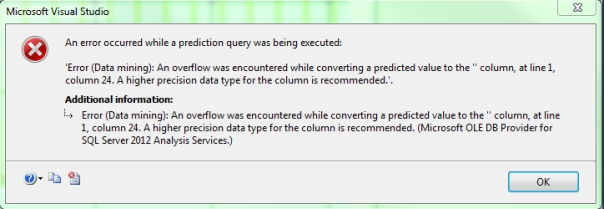
The Box-Jenkins Model provides a well-known methodology for combining them in a standard way that conserves enough information to make it useful for a wide range of projects. First the algorithm detects how stationary a data series is through a run sequence or auto-correlation plot, then calculates the differences between each interval and repeatedly adds terms to the equation until “statistical properties such as mean, variance, autocorrelation, etc. are all constant over time.”[xii] The point of this stage is to make the equation easier to work with. The greater the variability in the trends of a dataset, the more orders of difference will be necessary to smooth out the values, according to Books Online (BOL).[xiii] Normally in SSDM this requires a single difference order – which is why we typically see just one of them represented for each ARIMA node in the Generic Content Tree Viewer – but on occasion the algorithm will add a second difference order. This behavior can be changed by using two hidden parameters, ARIMA_AR_ORDER and ARIMA_DIFFERENCE_ORDER, which are cutting edge topics we won’t delve into at this point; we’re still walking up a creaky stairway in this series, not taking a space elevator. Seasonality, i.e. periodicity, is also detected through such means as auto-correlation or spectral plots. In Microsoft’s implementation, a common statistical tool called a Fast Fourier Transformation (which has been called “the most important numerical algorithm of our lifetime”) is applied to identify seasonality.[xiv] New terms are then added to the equation for each cyclical pattern detected in the data. Auto-correlation calculations are then applied to order the auto-regression and moving averages terms properly, by examining how well the data produced correlates with itself. This part of the calculation process is a bit opaque to an amateur like me, but at some point it may make use of least squares calculations, which we touched on briefly in A Rickety Stairway to SQL Server Data Mining, Algorithm 4: Logistic Regression. None of the concepts I’ve just glossed over are difficult to grasp, with the FFT being perhaps the most difficult. It took me three paragraphs to explain crudely how they are all combined together to output Time Series values though, which ought to give users an idea of just how many calculations are involved in the process. The number of calculation steps makes the algorithm relatively resource-intensive, so proper modeling and setting algorithm parameters correctly is of critical importance. There seems to be less risk of seeing the bogeyman of data mining, overfitting, in which poor performance is paired with cluttered, meaningless or misleading results, at least in comparison to other algorithms like Association Rules or Decision Trees. In my limited experience, I have seen far more problems with pure performance bottlenecks, which can crash SQL Server Analysis Services (SSAS) during the processing phase or SQL Server Data Tools (SSDT) when retrieving the mining results. Even when processing and retrieval are successful, it may take an inordinate amount of time to finish them. I have also received a couple of puzzling errors repeatedly in the SSDT and previous versions of Visual Studio on different Time Series projects, which thankfully don’t seem to affect the results returned in the GUI. One of the two error messages depicted below recommends that I use a data type of higher precision, but I still receive it when using the largest data types available in SSDM:
Figure 1: Frequent Time Series Error Messages in the GUI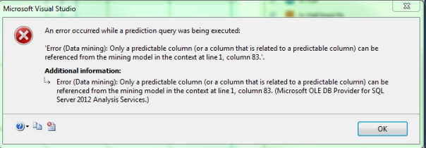
Throughout this series we’ve skipped using the NOT NULL and MODEL_EXISTENCE_ONLY mining flags, since our data has no nulls and there would be no advantage in reducing our data to a dichotomous choice of Missing or Existing states. Time Series has a unique MISSING_VALUE_SUBSTITUTION parameter that performs a related function, however, by filling in missing values in a prediction series with the Previous value, the Mean taken from moving averages during training or a specific number of your choosing. Leaving it at its default of None is a common source of model processing errors, especially with newly created mining models. Thankfully, Microsoft provides this crucial parameter in every edition of SQL Server. It may be important to set the other parameters of Time Series correctly to avoid performance problems and crashes, but beware, because many of them are only available in Enterprise Edition, like COMPLEXITY_PENALTY, HISTORIC_MODEL_COUNT, HISTORICAL_MODEL_GAP, INSTABILITY_SENSITIVITY, MAXIMUM_SERIES_VALUE, MINIMUM_SERIES_VALUE and PREDICTION_SMOOTHING. The DM Team’s aforementioned book says that MINIMUM_SUPPORT and COMPLEXITY_PENALTY are “rarely used” in versions after 2005 because of the addition of ARIMA, but I found it necessary to set them to non-default values in this week’s trials to avoid overfitting.[xv] As discussed in the tutorial on Decision Trees, these two parameters can be used to prune useless branches, but with ARTXP, the trade-off is not just between quality of results, model accuracy and performance, but in the stability of predictions, which tend to improve when these parameters are set more restrictively. In past projects I had trouble getting SSDM to return any results at all until I stumbled on a helpful post at Microsoft’s Data Mining Forum that explained how to set them correctly in a Time Series model. One of the problems discussed in that thread was alleviated by the addition of the INSTABILITY_SENSITIVITY parameter in SQL Server 2008, which allows users to turn off an internal inhibition on tree growth when the standard deviation of the predictions crosses a certain threshold. Since excessive tree growth is more of problem in this week’s trials and the parameter is only operative when the FORECAST_METHOD is set exclusively to ARTXP, I won’t get into a discussion of it here. I found it necessary to set the MINIMUM_SERIES_VALUE and MAXIMUM_SERIES_VALUE parameters, which limit the range of output values much like the common math functions Floor and Ceiling do in many programming languages. Unfortunately, they are set for entire models, not individual columns, which robs them of much of their usefulness. For example, if you’re predicting one series with a logical range of values between 100 and 1,000, and a second one that should range between 0 and 10, then the best you can do is set these parameters to 0 and 1,000 respectively. The first column can thus still produce values below its own natural floor, while the second can still output values above its natural ceiling.
The two seasonality parameters are indispensable though. When AUTO_DETECT_PERIODICITY is set closer to 1, it detects seasonal patterns more aggressively, with a corresponding risk of overfitting and possible reward of greater accuracy. The closer it is to zero, the less likely these three outcomes are. On several occasions I have found it useful to leave it set at its default of 0.6 and instead set PERIODICITY_HINT, which takes a comma-separated list of numerical values that you suspect occur at cyclical intervals in your data. A common use case might be to set it to {60, 24, 7} if you expect patterns to appear in your data by each minute in an hour, each hour in a day and each day in a week. You may track data by the minute, hour, day and week, yet that doesn’t necessarily mean that you should set periodicity hints for each of them. Unless your data tends to vary in a cyclical manner by those same intervals then there is no seasonality to detect. In that case SSDM even may ignore the hint, although this is unlikely, given that BOL says SSDM is “very sensitive” to it. For example, it might make sense to set it to 7 if you’re measuring sales at a restaurant which tends to do the same amount of business from one Monday to the next, but dissimilar amounts of business when comparing Monday’s sales to Saturday’s. In other business settings where sales are more uniform across a week, setting a periodicity hint of 7 would make less sense.
There are no parameters to control feature selection (which may not be used at all with Time Series, although it is difficult to tell from the documentation), nor is it advisable to set the three training holdout properties on each mining structure, since all you may be doing is deleting case data.[xvi] The closest equivalent Time Series has to training data are historical models, which are compared against each other to improve the accuracy of predictions. Since we have no future data to test the models on, we’re limited to using what’s already in our dataset. Testing a dataset against itself is of limited utility, since it’s practically tautological to gauge how well a model is trained solely by the training set it has already been fed. SSDM addresses this by dividing the data into separate models based on the HISTORIC_MODEL_COUNT parameter, which has defaults to a single model, then comparing them against each other. HISTORICAL_MODEL_GAP controls how they are divided, by truncating the data at the specified interval of time slices. The default is 10, but if you’re using it in tandem with HISTORIC_MODEL_COUNT, the goal is set it equivalent to the number of time slices you want to predict into the future.[xvii] As depicted in Figure 2, processing time roughly doubled between the third and sixth Time Series models, which had equivalent parameters except for HISTORIC_MODEL_COUNT, which was first set to its default then to 3. There was not much of a difference in performance for different HISTORIC_MODEL_GAP values. Oddly, performance decreased sharply when AUTO_DETECT_PERIODICITY was set to any value other than its default, regardless of whether it was lower or higher. Normally I test one variable at a time, but because of the extremely long processing times at the defaults, I set values for PERIODICITY_HINT, MINIMUM_SERIES_VALUE and MAXIMUM_SERIES_VALUE simultaneously and instantly received much better performance.
Figure 2: Performance Comparison for Various Trials of Time Series vs. Other Algorithms (click to enlarge)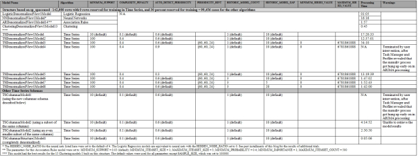
Before the trials depicted above, I was using an incorrect time key, which caused msmdrv.exe to load about a gigabyte and a half of RAM immediately in the initial trials, which later topped out at about 5 gigs. During that time the CPU seemed to run on one core, without much IO traffic at all. After I fixed that problem, SSAS ran on all six cores[xviii] most of the time and RAM usage rarely got above 600 megabytes, with no IO resource consumption. Processing was still time-consuming though, with the ARTXP phases seeming to take the longest. It’s always a good idea to monitor new SSDM projects in Profiler, but it is especially true with Time Series, which is aptly named because it can take quite a while to finish processing. During the ARIMA phases, you’ll see messages like “Learning ARIMA Time Series model for ‘MyColumn7′ in historical model number 1 (8 of 16)” repeated for each predictable column, first on the Main Model, then again for each historical model. Once you see messages like “Learning Time Series tree for ‘MyColumn5′ in main model (9 of 30)” then you’re in the ARTXP phase. The instances where msmdrv.exe got hung up for hours and I had to terminate the process manually seemed to occur most frequently during the ARTXP phase when building the trees for the Key Time columns, for whatever reason. I assume that the blending of the two algorithms takes place after this, but if so, it never contributed much to the final processing times. Some of the processing jobs took so long that it consumed much of the time I had set aside to write this post, so I limited my experiment to the mining structure built on sp_spaceused. As I discuss in more depth in past posts, the data used in these trials come from roughly three days of polling six dynamic management views (DMVs) every minute, in the hopes of creating IO pressure in order to study the topic further, as well as to use a type of data DBAs might be more familiar with. For a refresher on the schema we’ve basically stuck to throughout the series, see A Rickety Stairway to SQL Server Data Mining, Part 0.2: How to Dig Out of a Data Mining Cave-In. I did not dare run Time Series trials on the mining structures based on dm_os_wait_stats and dm_exec_query_stats, which had 7.6 million and 3.9 million rows respectively, plus many more columns with large data types.
I ran the first set of Time Series trials on those same denormalized schemas mainly for purposes of comparing its performance against a few select trials of other algorithms. Using a single denormalized view as the sole input table is not always the ideal way to design Time Series projects though. As I have tried to hammer home through this series, choosing the right Content type for your data is critical, because certain algorithms are limited in the ones that they will accept. Like Linear Regression, Time Series can work with Continuous attributes but not Discrete or Discretized ones; like all of the others except Sequence Clustering, it can accept Cyclical and Ordered data but simply treats them as Discrete values, rendering those Content types useless. Like many other algorithms, Time Series can use nested tables as both inputs and outputs, which may be useful in some projects depending on the natural schema of the data. The “key difference”[xix] is that Time Series requires a Key Time attribute to represent each unique time slice, which must come from a single numeric or date column. In other algorithms the case key is identified by the Key type, but it is optional with Time Series. In relational database lingo, it must have a 1:1 relationship with the Key Time column though. In previous projects I have used received quite good results using timestamps, such as single records for each day, as Key Time columns. In the first set of trials mentioned above, however, I was forced to use ID columns which were only roughly equivalent to proper time slices, thanks to such problems as the mysterious delays in the SQL Server Integration Services (SSIS) job that collected the data, which were recorded in the special MinuteGap column. To get results that would produce accurate projections of my data, rather than simple performance comparisons against other algorithms, a redesign of the schema seemed to be in order.
It was then that I finally understood the usefulness of the second Key, which I didn’t initially grasp from the written discussions on Time Series schemas in the DM Team’s book and Microsoft’s documentation.[xx] The algorithm can accept data in two ways, one of which is a columnar format, i.e. a normalized representation of data in which each Key Time represents a unique value. Unlike other algorithms, however, it can also be fed the same data in an interleaved format, in which each Key Time is not unique. Records in this somewhat denormalized format are identified through unique combinations of both the Key Time and Key columns, in a sort of composite key. The flexibility of the second approach is that users can add new values for whatever state the Key represents at will simply by appending new rows, whereas in the usual columnar approach a schema change would be required to add new columns to hold the new state value. On the other hand, it is not possible to use the new states as predictable attributes or set other mining structure properties if they’re not identified as separate columns. Perhaps the choice of the correct schema is highly dependent on whether or not you’re getting your data from a highly normalized relational database, like I am in these tutorials, or from the denormalized star or snowflake designs commonly used in cubes. The right choice probably also depends highly on whether or not all of the possible values for a state column are known, or whether they are subject to rapid change, as might be the case in a real-time OLAP scenario or one in which previously unseen values are generated frequently.. Because I learned the relational side of SQL Server first, (where “today’s new row is tomorrow’s new column”) my first instinct is usually to go with the most normalized approach – to the point that I found myself counting how many more cells it took to represent the same data in an interleaved format in the BOL and DM Team’s examples. Furthermore, I only have a few dozen columns to deal with rather than the several thousand used in real-world professional projects; if the schema was that large I’d probably be using a snowflake or star schema cube anyways. I thus made a quick redesign of the schema exclusively for this post, based on a columnar format in which I took a select few of the most important columns from the six DMVs the SSIS job collected data into. Using six ugly PIVOT statements, I put six of the most important performance counters in their own columns depending on whether they applied to All databases, the Monitoring database or TempDB; the nine tables I monitored using sp_spaceused received their columns, populated with their respective values for the Data column; one column was set aside for the io_stall values for the 25 unique FileHandleIDs in the dm_io_virtual_file_stats table; the nine most important wait types got their own columns; and each of the seven unique SchedulerAddress values from dm_io_pending_io_requests were given columns with their corresponding io_pending_ms_ticks values. Since we’re close to wrapping up the segment of this series that deals with the nine algorithms, I also used the unique groups of queries identified several weeks ago by the Clustering algorithm to create a new QueryTextGroupID column in my schema. For example, some of the queries fell into a particular cluster because they applied only to SQL Server Agent background tasks, while others applied to queries I made on the Monitoring database during data collection. I identified 25 of these distinct groups, each of which was filled with their respective values from the dm_exec_query_stats columns last_physical_reads and last_logical_writes added together. I also tossed in the mysterious MinuteGap column and a CombinedSmallDateTime column that collected all of the time measures in the RecordTable in a single Key Time attribute.
The results I received back from SSDM in this second set of trials were really quite interesting, although we don’t have time to go into them all. I gained a lot of insight throughout this series into how a real performance monitoring system might be properly built using SSDM, such as how to identify relationships between specific query types and various measures of IO, but never more than at the tail end of this final algorithm discussion. The main point of this series is though is to use this kind of data to illustrate how SSDM works – or how it doesn’t always work right, as was the case in my first few trials with this new schema. The first trial got hung up and the second only completed processing because I set many of the new columns to Ignore. Nevertheless, an old problem from the beginning of this series reared its ugly head again: the processing job finished, but the GUI was unable to retrieve the results without being hung up indefinitely, forcing me to terminate msmdrv after a few hours of waiting. This in turn crashed SSDT without warning. The same thing occurred after I removed many more columns in the third trial, even though there was substantial improvement in processing time. It wasn’t until I removed the nested table I had been using in favor of a single denormalized view that SQL Server was capable of representing the results in the GUI. Processing time also improved dramatically, to just over five minutes.
Figure 3: The Charts Tab with the Columnar Schema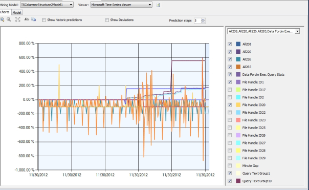
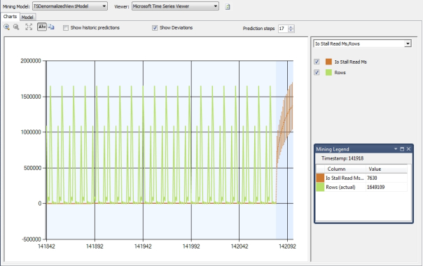
The run chart in Figure 3 would not be difficult to interpret, except for the fact that I found too many useful results and ended up cluttering it with too many columns. The date values at the bottom represent minute and hour figures as well as the day and date, but the GUI did not depict them in this case. Time moves forward as you go from left to right on the horizontal axis, while the values for the various columns increase or decrease by the percentages listed vertically on the left. The Abs button can be used to toggle between percentages and absolute values, which can harder to read if you have many columns with widely varied ranges of values. It is often wise to use the dropdown control on the right to select only a small subset of columns with similar ranges of values, otherwise those with smaller scales will be dwarfed by others in the run chart, regardless of their significance. The Prediction Steps dropdown can be used to control how far ahead the run chart peers into the future, up to a maximum of 100 intervals. On a few occasions I have had to close projects and reopen them before SSDT or Visual Studio would actually show the new predictions in the GUI, but I didn’t notice that bug in this week’s trials. Beware the Show Historic Predictions checkbox; it has always instantly crashed any version of SQL Server or Visual Studio I’ve ever used, without warning, regardless of the project. I vaguely recall seeing it work once or twice long ago, but I may be wrong; the most accurate prediction I can make in this post is that it will probably crash SSDT the next time I accidentally click on it. I’ll put that on the list of bugs I ought to submit to TechNet someday. Figure 4 shows how the Mining Legend depicts the time slice and values for two columns for whatever point the user clicks within the run chart, using data taken from the earlier set of trials performed on the sp_spaceused mining structure. Figure 5 shows the same data, except with the Show Deviations checkbox selected so that the variation of the data from the trend line is included in the regression lines.
Figures 4 and 5: The Chart Tab Mining Legend and Show Deviations Checkbox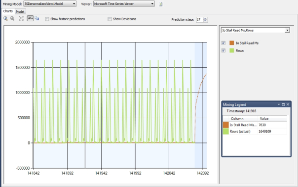
The Model Tab shows the ARTXP trees in a format very similar to the Decision Trees Viewer, which we have already discussed in detail and won’t explain again for sake of brevity. One of the few differences is that hovering over a node shows the ARIMA equation for the whole tree, which is the same for every node. Hovering over a leaf node also provides the tree equation, plus the coefficients and histograms in the Mining Legend. There is no Histograms dropdown, presumably because Time Series does not accept Discrete columns. As was the case with Decision Trees, the results are useful, but it some of the nonsensical relationships must be sorted out manually. For example, check out the comparisons for NumOfBytesWritten in Figure 6, which don’t tell us much. If NumOfBytesWritten is greater than or equal to a certain number, it’s not very useful to inform us that it is likely to be greater than or equal to another number in the following step. The output in this series did contain some useful splits, but I had to hunt for them.
Figure 6: The Time Series Model Tab (click to enlarge)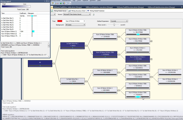
As always, if the information in the GUI is insufficient for your purposes, you can always dig deeper into the data with the Generic Content Tree Viewer. Because the output is so complex, I’ve included an example in Figure 7, in which there is one node in the tree to the left for each predictable attribute for ARTXP, and another row for each predictable attribute for ARIMA, with the ARTXP nodes at the top and the ARIMA ones at the bottom. Relating the ARTXP and ARIMA nodes would be an apples and oranges comparison, so don’t bother trying. There is one NODE_TYPE #16 for each predictable attribute, by followed by leaf nodes and/or interior branches, with leaf nodes at the end of any interior branch. There is also one NODE_TYPE #27 (i.e. an ARIMA Root) for each predictable attribute in ARIMA nodes, with multiple type #28 nodes for each periodic structure, each of which contains a single type #29 node for an auto-regression equation and a single type #30 for a moving average.
Figure 7: An Example of the Generic Content Viewer with the Times Series Algorithm (click to enlarge)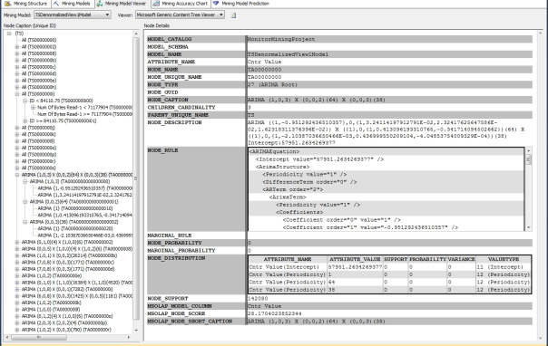
As usual, Time Series uses the same columns for its output that other algorithms do, but assigns different meanings to them. The meaning even varies from one row to the next, depending on its NODE_TYPE. As I have mentioned in the past, this denormalized structure is useful in the sense that it allows SSDM to represent the disparate output of its algorithms together, much like a produce stand can be used to hold both apples and oranges. The price to be paid for that is added complexity, thanks to the high level of denormalization, which also includes a nested NODE_DISTRIBUTION table in each row. Time Series uses the standard ATTRIBUTE_NAME, ATTRIBUTE_VALUE, SUPPORT, PROBABILITY and VARIANCE columns within it, but these can vary in meaning from one row to the next depending on their VALUETYPE flags. The NODE_DISTRIBUTION table is blank with ARTXP except in the leaf nodes, where the first row is always a VALUETYPE 11, for the Y-intercept. The rows that follow have a VALUETYPE of 7 for the coefficient or 9 for the Statistics. A lot of these concepts should already be familiar, given that we’ve already covered how they are depicted in the Generic Content Tree Viewer in the previous tutorials on Linear and Logistic Regression. Each NODE_TYPE #27 ARIMA root seems to have one VALUETYPE 11 row for the intercept, then one more for each NODE_TYPE #28 periodic structure within it. Each of the type #28s seems to have exactly one row apiece in its NODE_DISTRIBUTION table for periodicities, auto-regressive orders, difference orders and moving average orders, in that order. The SUPPORT, PROBABILITY and VARIANCE for all of these always seems to be 0, so the attribute-value pair is the distinguishing characteristic; this is true of both type #27 ARIMA roots and type #28 periodic structures. BOL says the complement of the coefficient is included in the data returned by the auto-regression, but I have yet to see it, unless the complement is the only value returned. It also says that it is possible to retrieve “the equation used to blend the algorithms,” but I have yet to find it.
Figure 8: Metadata for TS (adapted from Books Online as always – click to enlarge)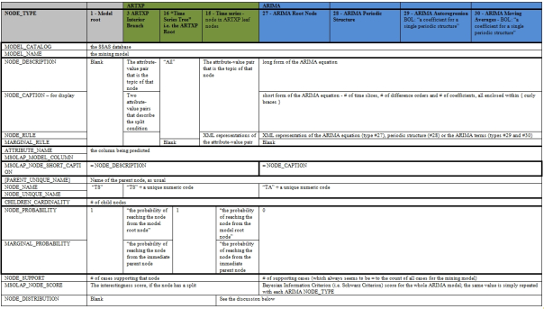
Obviously, I have much more to learn about the nine SSDM algorithms, particularly Sequence Clustering and Time Series. This is especially true when nested tables are involved, since they still seem to be my Achilles Heel. I’ve covered the basics of the algorithms sufficiently, however, that we can move on to the more advanced step of retrieving results directly through Data Mining Expression (DMX) queries. Instead of relying on the Generic Content Tree Viewer to tell us what we need to know, we can perform tasks like directly retrieving ARIMA equations or even reassembling ARTXP calculations, which BOL says can be difficult, “because information for each split is in a different place within the tree. Therefore, with an ARTXP model, you must get all the pieces and then do some processing to reconstitute the complete formula. Retrieving an equation from an ARIMA model is easier because the formula has been made available throughout the tree.” DMX can even be used to bypass the Generic Content Tree Viewer and other SSDM visualizations altogether, by exporting all of the data into other tools. In the fourth installment of our upcoming segment on DMX, I’ll explain how to import all of this denormalized data into a normalized relational database, where we can use T-SQL to slice and dice it with much greater ease. From there, it can even be imported into SSAS cubes, where it can be sifted through with Multidimensional Expressions (MDX). Both of these languages have far richer Data Manipulation Language (DML) capabilities than DMX, which is also quite limited in terms of its Data Definition Language (DDL). After several weeks of being force-fed a lot of thick information on some of SSDM’s most complex algorithms, the upcoming tutorials on DML and DDL should be a nice change of pace. In the third installment I will delve into the primary use for DMX, which is to perform prediction queries, particularly on Time Series data. There may be a delay in this series for a week or two while I recuperate from surgery for the antibiotic resistant sinus infection I mentioned back in December, but I don’t need Time Series to forecast that the lag will be short.
The new windowing functions in SQL Server 2012 can simplify the calculation of moving averages, as described in Ben-Gan, Itzik, 2012, Microsoft SQL Server 2012 High-Performance T-SQL Using Window Functions. O’Reilly Media, Inc.: Sebastopol, California.
[ii] I found the abbreviation at the blog of Jamie MacLennan, one of the leaders of Microsoft’s Data Mining Team in the last decade. See MacLennan, Jamie, 2007, “New Time Series Features for SQL Server 2008,” published Oct. 22, 2007 at Jamie’s Junk. Available at http://blogs.msdn.com/b/jamiemac/archive/2007/10/22/new-time-series-features-for-sql-server-2008.aspx
[iii] Meek, Chris; Chickering, David Maxwell and Heckerman, David, 2002 , “Autoregressive Tree Models for Time-Series Analysis,” published at the Microsoft Research website and available for download at http://research.microsoft.com/en-us/um/people/dmax/publications/dmart-final.pdf. Presented in the Proceedings of the Second International SIAM Conference on Data Mining (SIAM) at Arlington, Virginia, April 2002.
[iv] This done by setting multiple columns to Predict, which I have done throughout this series anyways regardless of the algorithm. For a short but enlightening discussion of cross-prediction, see Shuvro Mitra’s posts in the SQL Server Data Mining Forum thread “Time Series to Support Cross Prediction,” posted Oct. 28, 2008 at http://social.msdn.microsoft.com/forums/en-US/sqldatamining/thread/5a0d7196-9c1a-4ed6-b293-2d006042d5b2/
[v] p. 9, Meek, et al.
[vi] See the MSDN webpage “Mining Model Content for Time Series Models (Analysis Services – Data Mining)” at http://msdn.microsoft.com/en-us/library/bb677217.aspx
[vii] I’m paraphrasing a comment on p.12, Meek, et al.
[viii] p. 282, MacLennan, Jamie; Tang, ZhaoHui and Crivat, Bogdan, 2009, Data Mining with Microsoft SQL Server 2008. Wiley Publishing: Indianapolis.
[ix] Jenkins “was a jazz and blues enthusiast and an accomplished pianist,” according to the Wikipedia webpage “Gwilym Jenkins” at http://en.wikipedia.org/wiki/Gwilym_Jenkins. Any statistician who can jam is a friend of mine. Box’s work during the war may seem repellent in the present age, now that chemical weapons are taboo and groups like PETA protect animal rights so rabidly, but at the time there was considerable fear that Hitler would use chemical weapons against Britain. So I would not include him in the long list of mathematicians and professionals in the hard sciences who have gone mad, wasted their talents on junk science or became terrible philosophers, as I have mentioned throughout this series. That might apply, however, to critics who base their censure on the inhuman idea that animal life is worth as much as human life. See the Wikipedia webpage “George E. P. Box” at http://en.wikipedia.org/wiki/George_Box
[x] See the Wikipedia webpage “Autoregressive–moving-average model” at http://en.wikipedia.org/wiki/Autoregressive_moving_average_model. Also see Box, George E.P. and Jenkins, Gwilym M., 1971, Time Series Analysis: Forecasting and Control. Holden-Day: San Francisco. I have not had the chance to read the latter yet.
[xi] For further background, also see the Wikipedia webpages “Box–Jenkins” at http://en.wikipedia.org/wiki/Box%E2%80%93Jenkins, “Corellogram” at http://en.wikipedia.org/wiki/Autocorrelation_plot and “Autocorrelation” http://en.wikipedia.org/wiki/Autocorrelation
[xii] For a quick explanation of differencing, see Prof. Bob Nau’s notes for the Forecasting – Decision 411 course at the Duke University webpage titled “Stationarity and Differencing,” available at http://people.duke.edu/~rnau/411diff.htm
[xiii] See the MSDN webpage “Microsoft Time Series Algorithm Technical Reference” at http://msdn.microsoft.com/en-us/library/bb677216.aspx
[xiv] p. 282, MacLennan, et al. For the comment about the FFT, see See Strang, Gilbert, 1994, “Appendix I: Wavelets,” pp. 250-255 in American Scientist No. 82, April, 1994. I’m not sure what version of the FFT is used by SSDM, but the most common one is the recursive Cooley-Tukey algorithm. See the Wikipedia webpage “Fast Fourier Transform” at http://en.wikipedia.org/wiki/Fast_Fourier_transform.
[xv] IBID., pp. 288-289.
[xvi] IBID., p. 271.
[xvii] IBID., pp. 287-288.
[xviii] My poor beat-up development machine uses an AMD CPU. Microsoft’s documentation warns that SSDM can return quite different results for Itanium processors when they are fed the same datasets, thanks to their notorious floating point processing problem. I can’t comment on that issue because I have never run on SSDM on an Itanium machine.
[xix] Pun intended.
[xx] See the MSDN webpage “Microsoft Time Series Algorithm” at http://msdn.microsoft.com/en-us/library/ms174923.aspx. Also see pp. 265-266, MacLennan, et al.


